Week 4 - Genetic Algorithm
Aim : To write a code to calculate the global maxima using genetic algorithm, by using a matlab.
Genetic algorithm : A genetic algorithm is a search heuristic that is inspired by Charles Darwin's theory of natural evolution. This algorithm reflects the process of natural selection where the fittest individuals are selected for reproduction in order to produce offspring of the next generation.
Genetic algorithm uses :Genetic algorithms are commonly used to generate high-quality solutions to optimization and search problems by relying on biologically inspired operators such as mutation, crossover and selection.
Genetic works : The following outline summarizes how the genetic algorithm works The algorithm begins by creating a random initial population. The algorithm then creates a sequence of new populations. At each step, the algorithm uses the individuals in the current generation to create the next population.
Genetic algorithm examples :Genes will be subjected to crossover at selected positions in the chromosome. For example, if the chromosome is [1,1,0,1,1,0,0,1] and position is 2 (from left). Then the value 1 will be replaced with mating chromosome's value at the same position.
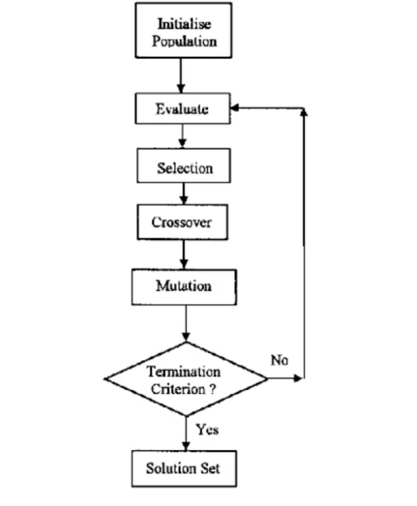
Five phases are considered in a genetic algorithm.
- Initial population
- Fitness function
- Selection
- Crossover
- Mutation
Optimization : attempts at solving optimization problems on computers. “Programming,” with the meaning of optimization, survives in problem classifications such as linear .
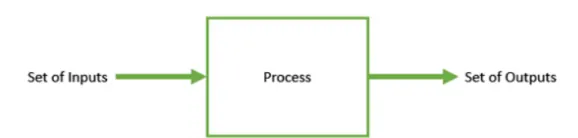
The purpose of optimization is to achieve the “best” design relative to a set of prioritized criteria or constraints. These include maximizing factors such as productivity, strength, reliability, longevity, efficiency, and utilization.
Producere :
>The defining the our search space, and the required inputs of x,y are the inputs commands.
> then these inputs of aary vectors [xx,yy],so than can u evaluated the function of two variables and plot the 2dimensional mesh/surface
>then i know of to minimus inputs, to finding the minimus of inputs lets give out of defining the function.(f)
>now, the x and y are the inputs vector of function ,now the parameter num_cases,and f function are generated the stalagmite function,just calling a ‘ga’,and optimum value products the function ,then i stored the values of xopt,and yopt,values and finding out of it fopt.
>look at the stalagmite function i created plot on the surface(x,y,f).while ‘ga’ which helps of how algorithms performance and we should clear the little bit of plot used of the subplot again.and directly function of x- axis iteration and y -axis function minimus.during the iteration the value of changes this is not importance.
>u saw in the graph of above study the x-axis and y -axis below zero and above the one in the axis of point given range 0.6.
>By using, the explain of ga syntax words of study time(1).study time(2).and finally of study time (3).
>study one,the Ga is does not run the with particular search space,since we not defined the bound.
>x is the local minima point
>fun is the called function (in case, it is stalagmite function)
>nvars indicated the no of variables used.
>study(2)here,the upper and lower bounds are defined so as to know the boundaries which within global maxima lies.
>x is the local minima point
>fun is the called function (in case, it is stalagmite function)
>nvars indicated the no of variables used.
>A and B are used to indicates any kind of inequalities that exist in the function.
>lb is indicates the lower bound
>ub is indicates the upper bound
>study(3),the population size is increased
>x is the local minima point
>fun is the called function (in case, it is stalagmite function)
>nvars indicated the no of variables used.
>A and B are used to indicates any kind of inequalities that exist in the function.
>lb is indicates the lower bound
>ub is indicates the upper bound
>nonlcon gives a two vector representing the inequalities and equalities
>options is used to perform additional operation like increasing the population size.this done with help of ‘optiomoption’.
>And under same of figure(1),figure(2)and figure(3) are accordingly
>plot
>title
>subplot
>xlabel(iteration)
>ylabel('function maxima)
>And print of sprint% gobal max optimised function value
The format of genetic alogarithm in a MATLAB,as follows

cases study (2);
x = is the local minima point
f = is the called function (STALAGMITE FUNCTION)
objective function is stalagmite and the number of variable is 2
A,B,Aeq and Beq = [],as ther is no linear equalities and in equalities in this function.
lb = lower bound of variable x and y in 'ga' algorithm is set as [0'0]
up = upper bound of variable x and y in 'ga' algorithm is set as [1,1]
same,cases(3):
x = is the local minima point
f = is the called function (STALAGMITE FUNCTION)
objective function is stalagmite and the number of variable is 2
A,B,Aeq and Beq = [],as ther is no linear equalities and in equalities in this function.
lb = lower bound of variable x and y in 'ga' algorithm is set as [0'0]
up = upper bound of variable x and y in 'ga' algorithm is set as [1,1]
options = increasing the population size 300
CODE:
clear all
close all
clc

%defining the our sreach space
 x = linspace(0,0.6,150);
 y = linspace(0,0.6,150);
 num_cases = 200

  [xx,yy] = meshgrid(x,y);

 for i = 1:length(xx);
     for j = 1:length(yy);
      input_vectors(1)=xx(i,j);
      input_vectors(2)=yy(i,j);
      f(i,j)=stalagmite(input_vectors);
     end
 end
 %study 1
 tic
 for i = 1:num_cases
     [inputs,fopt(i)] = ga(@stalagmite,2);
     xopt(i) = inputs(1);
     yopt(i) = inputs(2);
 end

 study1_time = toc;
  figure(1)
 subplot(2,1,1);
 hold on
 f1 = -f       %ga gives the minima value,inverse of -f is taken maxima value
 surfc(xx,yy,f1);
 shading interp
 fopt1 = -fopt;
 plot3(xopt,yopt,fopt1,'marker','o','markersize',5,'markerfacecolor','r');
 title('unbounded inputs');
 subplot(2,1,2);
 plot(fopt);
 xlabel('Iteration');
 ylabel('function maxima');


 %study2
 tic
 for i = 1:num_cases
     [inputs,fopt(i)] = ga(@stalagmite,2,[],[],[],[],[0;0],[1;1]);
     xopt(i) = inputs(1);
     yopt(i) = inputs(2);
 end

 study2_time = toc;
 figure(2);
 subplot(2,1,1);
 hold on
 f2 =-f;
 surfc(xx,yy,f2);
 shading interp;
 fopt2 = -fopt;
 plot3(xopt,yopt,fopt2,'marker','o','markersize',5,'markerfacecolor','r');
 title('with bounded inputs');
 subplot(2,1,2);
 plot(fopt);
 xlabel('Iteration');
 ylabel('function maxima');


 %study3 increasing Ga iteration;
 options = optimoptions('ga');
 options = optimoptions(options,'populationsize',300);

 tic
 for i = 1:num_cases;
     [inputs,fopt(i)] = ga(@stalagmite,2,[],[],[],[],[0;0],[1;1],[],[],options);
     xopt(i) = inputs(1);
     yopt(i) = inputs(2);
 end

 study3_time = toc;
  figure(3);
 subplot(2,1,1);
 hold on;
 f3 = -f ;
 surfc(xx,yy,f3);
 shading interp;
 fopt3 = -fopt;
 plot3(xopt,yopt,fopt3,'marker','o','markersize',5,'markerfacecolor','r');
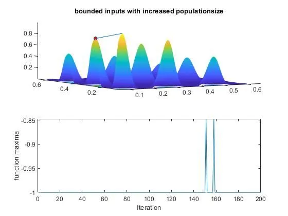
 title('bounded inputs with increased populationsize');
 subplot(2,1,2);
 plot(fopt);
 xlabel('Iteration');
 ylabel('function maxima');

 fprintf('\n The Global max optimised function Value %f',fopt3);
The function:
%the function of fiding the input minimus
function [f] = stalagmite(input_vectors)

x =  input_vectors(1);
y =  input_vectors(2);

f1=(sin(5.1*pi*x+0.5))^6;

t= ((x-0.0667)^2/0.64);
t1= ((y-0.0667)^2/0.64);

f2 = exp(-4*log(2)*t);


f3 = (sin(5.1*pi*y+0.5))^6;

f4 = exp(-4*log(2)*t1);


f = -(f1*f2*f3*f4);
end
to defing iteration the study (1),the Ga is does not run the with particular search space,since we not defined the bound.
%defining the our sreach space
 x = linspace(0,0.6,150);
 y = linspace(0,0.6,150);
 num_cases = 200

  [xx,yy] = meshgrid(x,y);

 for i = 1:length(xx);
     for j = 1:length(yy);
      input_vectors(1)=xx(i,j);
      input_vectors(2)=yy(i,j);
      f(i,j)=stalagmite(input_vectors);
     end
 end
 %study 1
 tic
 for i = 1:num_cases
     [inputs,fopt(i)] = ga(@stalagmite,2);
     xopt(i) = inputs(1);
     yopt(i) = inputs(2);
 end

 study1_time = toc;
  figure(1)
 subplot(2,1,1);
 hold on
 f1 = -f       %ga gives the minima value,inverse of -f is taken maxima value
 surfc(xx,yy,f1);
 shading interp
 fopt1 = -fopt;
 plot3(xopt,yopt,fopt1,'marker','o','markersize',5,'markerfacecolor','r');
 title('unbounded inputs');
 subplot(2,1,2);
 plot(fopt);
 xlabel('Iteration');
 ylabel('function maxima');
In the iteration,study(2)here,the upper and lower bounds are defined so as to know the boundaries which within global maxima lies.
%study2
 tic
 for i = 1:num_cases
     [inputs,fopt(i)] = ga(@stalagmite,2,[],[],[],[],[0;0],[1;1]);
     xopt(i) = inputs(1);
     yopt(i) = inputs(2);
 end

 study2_time = toc;
 figure(2);
 subplot(2,1,1);
 hold on
 f2 =-f;
 surfc(xx,yy,f2);
 shading interp;
 fopt2 = -fopt;
 plot3(xopt,yopt,fopt2,'marker','o','markersize',5,'markerfacecolor','r');
 title('with bounded inputs');
 subplot(2,1,2);
 plot(fopt);
 xlabel('Iteration');
 ylabel('function maxima');
In the iteration,study(3)the population size as is increased
 %study3 increasing Ga iteration;
 options = optimoptions('ga');
 options = optimoptions(options,'populationsize',300);

 tic
 for i = 1:num_cases;
     [inputs,fopt(i)] = ga(@stalagmite,2,[],[],[],[],[0;0],[1;1],[],[],options);
     xopt(i) = inputs(1);
     yopt(i) = inputs(2);
 end

 study3_time = toc;
  figure(3);
 subplot(2,1,1);
 hold on;
 f3 = -f ;
 surfc(xx,yy,f3);
 shading interp;
 fopt3 = -fopt;
 plot3(xopt,yopt,fopt3,'marker','o','markersize',5,'markerfacecolor','r');
 title('bounded inputs with increased populationsize');
 subplot(2,1,2);
 plot(fopt);
 xlabel('Iteration');
 ylabel('function maxima');

 fprintf('\n The Global max optimised function Value %f',fopt3);
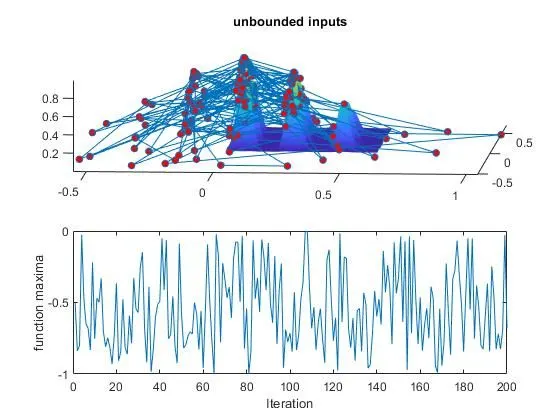
Plot the 1st iteration(iteration = 200),by obtaining the using of 'ga'
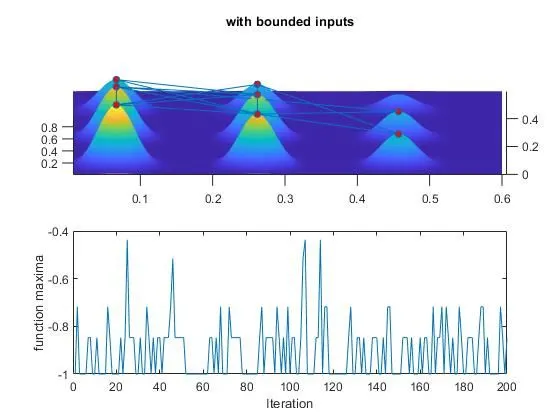
plot the 2 iteration
plot the 3iteration(iteration 200,population300)
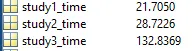
the above given of the cases study of(1, 2, 3)of study time changes.
Results:
1)in the above image it can be seen that the inputs are boundariless, ga algorithm is placced of maxima value of out side the stalagmite function. so its not of clearness and its of use of pointless.
2)In the 2nd plot the boundary conditions are specified using the upper and the lower bounds, with a fixed number of iterations.
3) In the last plot we clearly see that the boundary conditiona are specified along with the population size of 170. Here we see the least deviation and the ga can perform the operation with max optimisation.
Note :- The max function value of the ga is 1 as the function rule states that `f max = -(f min)`