Week 3 - Solving second order ODEs

AIM: To solve the second-ord simulate the transient motion of a simple pendulum and a creation of animation of motion

Governing equation:

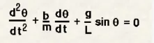..............(1)

The above equation of finding the ode solver to calculating the angular displacement given by (theta).

Angular displacement:Angular displacement of a body is the angle in radians (degrees, revolutions) through which a point revolves around a centre or line has been rotated in a specified sense about a specified axis.Thus the rotation of a rigid body over a fixed axis is referred to as rotational motion.

The SI units of angular displacement,RADIAN OR DEGREE.

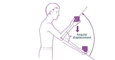
Simple pendulum: A simple pendulum is a mechanical arrangement that demositarts periodic motion . the simple pendulum comprises a small bob of mass “m”.

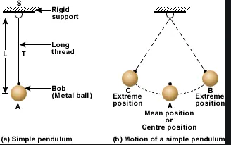
EXPLANATION:

The given equation of

Here as : b = damping

m= mass

g = gravity

l = length

To solve the second-order function in the second order is to not calculate it, we should convert the equation in first order.

Let the

..........(2)

and,if `theta1`change with respect to time we can say that

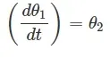.............(3)

Aslo,we can say that

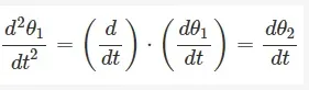...............(4)

Now,by substituting equation (3) and (4) in equation (2),we get

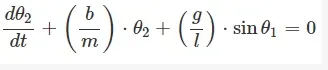............(5)

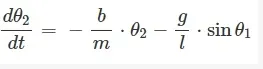..............(6)

By,using the equation (3) and (4) which of is first order we will simulated the simple pendulum by using the MATLAB.

PROCEDURE:

It is better to start programming in matlab with these three commands as through these all the previous calculation is erased.

Clear all : this command clear all the data stored in the workspace previously

Close all : this command closes all the previous figure and plots

Clc : this command clears the command window.

Now, create all the variable required,

b = 0.05

g = 9.81

L = 1

m = 0.1

Here the two first-order odes are the dtheta_1and dtheta_2

Use,the ode 45 solve the ode function

(t,results) = ode45(t,theta)ode fun_second_order_(theta,b,g,l,m) t_span,theta(0);

Now, plot the results theta1 and theta2 against it will give a plot of displacement vs velocity.

Now, create the animation,

The give of valves of (x1,y1)think of assume axis(-5,0) and(x2,y2)axis(5,0)where axis of center of simple pendulum horizontal line origin(x3,y3)axis (0,0) and finally the axis of pendulum ball of displacement are the (x4,y4)axis(x4sintheta,y4 -costheta)

Now allocating the coordinates of fixed support,now plot (0,0) and ‘o’ as the markersize

Now allocating the coordinate for the pendulum string.plot(0,x)and(0,y)

Now allocating the coordinate for the BOB.or BALL

Now, create the movie,

movie(M),

video File =videowriter(‘ode.avi’,’uncompressed AVI)

open(video file)

writevideo(video file M)

close(video file)

CODE:

clear all
close all
clc 


b = 0.05;
g = 9.81;
l = 1;
m = 0.1;

%initial condition
   theta_0 = [0;5];
   
   
%time points 
  t_span = [0 20]
  
  
  %slove ODE
  [t,results] = ode45(@(t,theta) odefun_second_order_nishanth(theta,b,g,l,m),t_span,theta_0);
  
  figure(1)
  plot(t,results(:,1))
  hold on
  plot(t,results(:,2))
  xlabel ('Velocity')
  ylabel ('displacement')
  legend( 'angular displacement','angular velocity')
  
  ct=1


for i=1:length(results(:,1));
 x=-1*sin(results(i,1));
 y=-1*cos(results(i,1));

 figure(2)

 
 plot(0,0,'o','Markersize',10,'color','b','Markerfacecolor','b') %allocting co-ordinates for fixed support
 plot([0 x],[0 y],'linewidth',2,'color','b') %allocting co-ordinates for pendulum string
 hold on
 plot(x,y,'-o','markers',10,'markerfacecolor','r') %allocting co-ordinates for BOB
 xlim([-1.5 1.5]);
 ylim([-1.5 1.5]);
 grid on

 pause(0.002);
 hold off
 M(ct)= getframe(gcf);
 ct=ct+1;
end

movie(M)
videofile = VideoWriter('ode.avi','Uncompressed AVI');
open(videofile)
writeVideo(videofile,M)
close(videofile)

FUNCTION:

function[theta_dot]=odefun_second_order_nishanth(theta,b,g,l,m)
    

    
%Rate of change of displacement= velocity
  
theta_dot(1)=theta(2);

theta_dot(2)=((-b/m)*theta(2))-((g/l)*sin(theta(1)));
theta_dot=[theta_dot(1);theta_dot(2)]
end

PLOT:

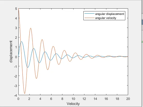
ANIMATION: Pendulum

CONCLUSION: By the simple pendulum,as the displacement and velocity was decrease, the damping force increases.