Week 4 - Genetic Algorithm
Genetic Algorithm in Matlab
Aim:
To understand the concept of genetic algorithm and to find the way to optimize the stalagmite function to find it’s global maxima.
Objective:
To write a Matlab code to optimize the stalagmite function to find the global maxima under 3 conditions as below
- Optimize stalagmite function and plot graph for Study-1 Unconstrained optimization
- Optimize stalagmite function and plot graph for Study-2 Optimization with lower and upper bounds
- Optimize stalagmite function and plot graph for Study-3 Optimization with lower, upper bounds and population size
Stalagmite function over view:
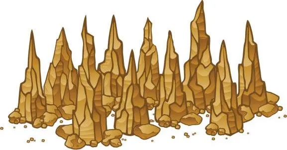
Stalagmite is the mineral formation found in caves. Where water drips down onto the floor, over and over on the same spot. The water evaporates, leaving any minerals in it behind. Those minerals pile up over time and solidify into rock. Over many years, they will form a rock mound on the floor which is called as stalagmite.
The mathematical function that governs the stalagmite shape is as below
`f(x,y)=f_1x f_2x f_1y f_2y`
Where,
`f_1x=[sin(5.1πx+0.5)]^6`
`f_1y=[sin(5.1πy+0.5)]^6`
`f_2x=exp[-4ln(2)(x-0.0667)^2/0.64]`
`f_2y=exp[-4ln(2)(y-0.0667)^2/0.64]`
The above function yields the stalagmite model with local minima and global maxima like in the below depicted picture.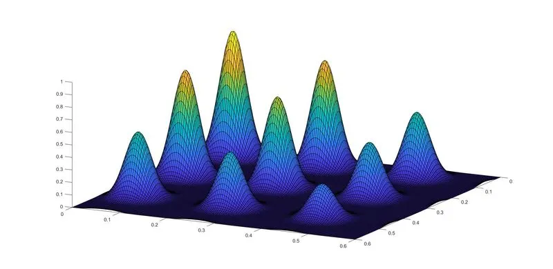
Optimizing Stalagmite function:
Here our aim is to optimize the stalagmite function to find it’s global maxima. Optimization in terms we have to find the exact input that could lead to the optimum point.
The one way to find the optimum value is the introduction of Genetic algorithm concept in to the analysis which can find the minimum value of the function which is generally the optimum value in any system, but still the stalagmite function can be modified in such a way that could help us to find the global maxima.
In general the genetic algorithm concept intended to find the least possible value of a function.by inverting the stalagmite function yield it may search further down in to finding the least value with could be a negative value below zero.To attain this, the stalagmite function can be modified as below by inverting the function using the negation operator.
`f(x,y)=-f_1x f_2x f_1y f_2y`
Genetic algorithm overview:
Genetic Algorithm (GA) is a search-based optimization technique using the principles of Genetics and Natural Selection. It is used to find optimal or near-optimal solutions to difficult problems these techniques are most widely used in research sectors.
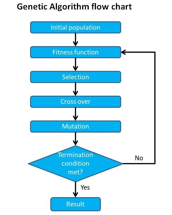
The genetic algorithm functions by the steps below
- Initial population
- Fitness function
- Selection
- Cross over
- Mutation
- Termination
- Initial population:
Genetic algorithm starts with the set of individual called initial population, each individuals are the solution for the problem.
Individuals here have different characteristics which have to be swapped during the process of genetic algorithm. Population size contributes much to the better optimization result. - Fitness function:
Fitness function the function used to evaluate the fitness of the individual.
based on the fitness score the individual can be selected for process of GA. - Selection:
Selection is the step where the fittest individual getting selected to carry over their characteristics to the next generation.
Pair of individual gets selected based on the fitness score they obtain. - Crossover:
At this process the individual partially swaps their characteristics with one another to produce offsprings of combined characteristics.
A cross over point would be chosen at which the set of different characteristics of the individual would be swapped to produce the new offsprings. The new offsprings will be then added in to the population as the next generation. - Mutation:
Mutation is the process at which the any one of the characteristic of the offsprings will be getting flipped. This process takes place randomly.
Mutation occurs to introduce diversity among the population to avoid the convergence when still there is room for new generations. This helps to get more precise result of optimization. This process repeats until the population converges. - Termination:
Termination is final stage where the algorithm stops. i.e. the process does not produces offsprings which are different from the previous generation. The process would not have a way to carry on the generations with significant diversities.At this time it can be said that the process provided a solution for the problem.
Genetic Algorithm in Matlab:
Matlab has an inbuilt function for genetic algorithm to solve complex problems by the name GA. Which helps to find the minimum of a function.
GA Syntax:
There are different GA syntax available in matlab for different nature of problems, the syntax are as given below.
- x= ga(problem) finds the minimum for problem, a structure described in problem can be any kind of problem with the parameters as listed below.
- x = ga(fun,nvars)
here the GA find the local minimum x at unconstrained condition. To perform this command the GA need the fitness function and the number of variables that the function could consume. - x = ga(fun,nvars,A,b)
The GA here finds the local minimum of the function subjects to linear inequality constraints have the form A·x ≤ b. When Ais m-by-n, there are m constraints on a variable x with n components. - x = ga(fun,nvars,A,b,Aeq,beq)
The GA finds the local minimum of the function subjects to linear equalities of form Aeq·x = beq and inequalities A·x ≤ b. if there is no linear inequalities then A and b have to be se to A=[] and b=[] respectively. - x= ga(fun,nvars,A,b,Aeq,beq,lb,ub)
The GA finds the local minimum of the function with boundary constraints.
in addition to the set of linear equalities and inequalities if applies it adds a set of upper and lower boundaries for the function in the form lb ≤ x ≤ ub. If there don’t exist the linear or non-linear inequalities then A,b,Aeq and beq can be set as A=[],b=[], Aeq=] and beq=[]. - x= ga(fun,nvars,A,b,Aeq,beq,lb,ub,nonlcon)
This leads the function minimization by subjecting it through the function handlenonlcon. Where nonlcon is non linear constraints.nonlcon is a function that accepts a vector or array x and returns two arrays, c(x) and ceq(x) as non linear equalities and non linear equalities respectively, where the GA attempts to satisfy the condition c<= 0 for all c and ceq= 0 for all ceq.if there is no need for upper and lower bounds then those can be set to lb=[] and up=[]. - x= ga(fun,nvars,A,b,Aeq,beq,lb,ub,nonlcon,options)
This minimizes the function by where any additional constraint parameter can be added through Here in our study we have inserted the population size in to the GA through options. Any non linear condition can be left unspecified by setting nonlcon=[]. - x= ga(fun,nvars,A,b,[],[],lb,ub,nonlcon,IntCon)
This minimizes the function under the condition with any variable present in the Intcon will take part as integer values.
nteger variables, specified as a vector of positive integers taking values from 1 to nvars. Each value in IntCon represents an x component that is integer-valued.
To use the integer variable there are restrictions that any linear equalities Aeq, beq must be empty and the the non linear constraint (nonlcon) must return empty value for ceq. - [x,fval] = ga(___)
The GA minimizes the function and returns the input arguments and the value of the fitness result at given x. - [x,fval,exitflag,output] = ga(___)In addition to the input arguments and the fitness result the GA also returns the exitflag, which is the termination reason for which the algorithm got stopped. Along with that the GA also returns output, that is the structure that contains the output from each generation and other information about the algorithm performance such as problemtype, evaluation count, number of generation, maximum constraint violation,etc,.
- [x,fval,exitflag,output,population,scores] = ga(___)
Here the GA also returns a population matrix where the number of rows are the number of individual of the population. And it returns the final score, The final scores are the fitness function values for the returned rows of population.
Matlab code to optimize stalagmite function:
Fitness function:
Here is the stalagmite fitness function for which the GA going to optimize the global maxima of the model. The input arguments from the main function will be passed on to the fitness function as x and y values.
For any function the GA attempt to find the minimum of the function, in our case our intention is to find the global maximum of the function, so the stalagmite function has been modified in such a way to find the maximum by adding negation to the output result of the function. Now the function will attempt to find the minimum value further low, which is a negative value.
%Stalagmite function
function [f]=stalagmite(input_vector)

x=input_vector(1);                         %Input for function
y=input_vector(2);                         %Input for function

f1x=(sin((5.1*pi*x)+0.5))^6;
f1y=(sin((5.1*pi*y)+0.5))^6;
f2x=exp((-4*log(2)*(x-0.0667)^2)/0.64);
f2y=exp((-4*log(2)*(y-0.0667)^2)/0.64);

f=-(f1x*f2x*f1y*f2y);                       %Inverting the function to find global maxima

end
Study-1:
Unconstrained optimization
Code explanation:
The GA attempts to optimize the stalagmite fitness function to find the global maxima without any constraints.
- For this code the search space has been declared from 0 to 0.6 with 150 units for both x and y inputs. And iteration has been set to 100.
- The search space vectors x and y has been converted in to matrix form using the meshgrid command.
- The input arguments for the fitness function will be generated using for loop and nested for loop over each element of the matrix picked up as ‘i’ and ‘j’ values as input_vector(1) and input_vector(2).
This in turn computes the fitness value of the stalagmite function. - As we know that we have inverted the stalagmite function to find the most minimum value which is a negative value which would also flip the stalagmite model. So we have inverted the fitness result by adding a negation operator in the main function.
- The GA optimization for the function will be carried out in this step.
To find the close optimal result the GA optimization will be executed for the number of times as per the iteration value provided as 100.
The optimization starts with the GA syntax based on x = ga(fun,nvars).
We have modified the syntax in a way to return the input arguments and the fitness result as [inputs,Fopt(k)]=ga(@stalagmite,2). - The result is then plotted using subplot
In subplot-1 stalagmite model has been plotted as surface using surf command and the GA optimum points are plotted using plot3 command, which is a 3D plotter.
In subplot-1 the optimum results for each iteration has been plotted respectively. - Timer has been introduced to calculate the optimizationtime using the tic and toc command.
Code:
clear all
close all
clc

%Study-1 unconstrained Optimization
%Search space
x=linspace(0,0.6,150);
y=linspace(0,0.6,150);
Iteration=100;                         %Number of iterations
[xx,yy]=meshgrid(x,y);

%Input for stalagmite function
for i=1:length(xx)
    for j=1:length(yy)
        input_vector(1)=xx(i,j);
        input_vector(2)=yy(i,j);
        f(i,j)=stalagmite(input_vector);
    end
end
f=-f;                                 %To invert the surface plot


%Function optimization for the given iteration
tic
for k=1:Iteration
[inputs,Fopt(k)]=ga(@stalagmite,2);
xopt(k)=inputs(1);
yopt(k)=inputs(2);
end
toc
Fopt=-Fopt;                           %To invert the optimum point

%Plotting
figure(1)
subplot(2,1,1)
surf(xx,yy,f)
title('Optimization-Unconstrained')
xlabel('X-axis')
ylabel('Y-axis')
zlabel('Fopt')
shading interp
hold on
plot3(xopt,yopt,Fopt,'marker','o','markersize',5,'markerfacecolor','r')
subplot(2,1,2)
plot(Fopt)
title('Optimization-Unconstrained')
xlabel('Iteration')
ylabel('Fopt')
Result: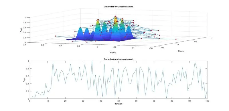
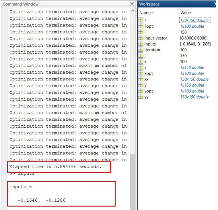
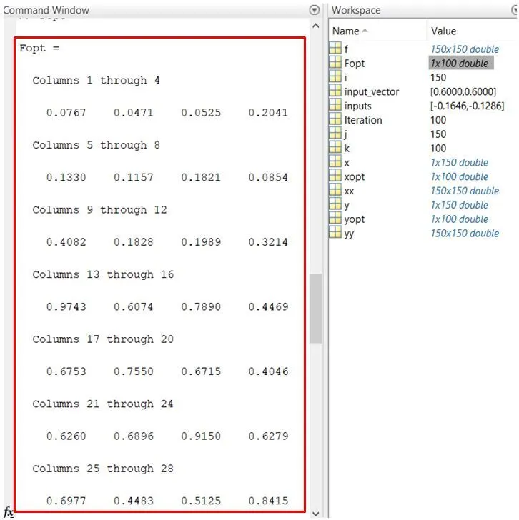
Due to the unconstrained condition the global maxima seems to have more deviation during the execution on each iteration.
Study-2:
Optimization with lower and upper bounds
Code explanation:
- For study-2 it has been provided with the same search space and iteration like for study-1. Which evaluates the same stalagmite fitness function with the input vectors.
- A for loop has been introduced for the number of iteration, inside of which a GA function based on syntax x= ga(fun,nvars,A,b,Aeq,beq,lb,ub) has been declared to constrain the function with the lower and upper boundaries.
We have modified the syntax in such a way to return the input and the Fopt values as before. The modified the GA syntax is given as [inputs,Fopt(k)]=ga(@stalagmite,2,[],[],[],[],[0;0],[0.6;0.6]); this calls the stalagmite function and compute with lower and upper boundaries, the empty cells represents the absence of linear and non linear inequalities. - The result has been plotted in the same way as study-1.
Code:
clear all
close all
clc

%Study-2 Optimization with upper and lower bounds
%Search space
x=linspace(0,0.6,150);
y=linspace(0,0.6,150);
Iteration=100;                               %Number of iterations
[xx,yy]=meshgrid(x,y);

%Input for stalagmite function
for i=1:length(xx)
    for j=1:length(yy)
        input_vector(1)=xx(i,j);
        input_vector(2)=yy(i,j);
       f(i,j)=stalagmite(input_vector);
    end
end
f=-f;                                      %To invert the surface plot


%Function optimization for the given iteration
tic
for k=1:Iteration
[inputs,Fopt(k)]=ga(@stalagmite,2,[],[],[],[],[0;0],[0.6;0.6]);
xopt(k)=inputs(1);
yopt(k)=inputs(2);
end
toc
Fopt=-Fopt;                               %To invert the optimum point

%Plotting
figure(1)
subplot(2,1,1)
surf(xx,yy,f)
title('Optimization with upper and lower bounds')
xlabel('X-axis')
ylabel('Y-axis')
zlabel('Fopt')
shading interp
hold on
plot3(xopt,yopt,Fopt,'marker','o','markersize',5,'markerfacecolor','r')
subplot(2,1,2)
plot(Fopt)
title('Optimization with upper and lower bounds')
xlabel('Iteration')
ylabel('Fopt')
Result: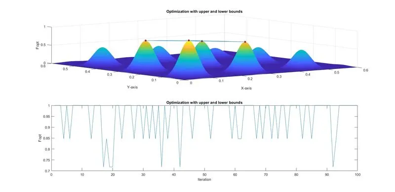
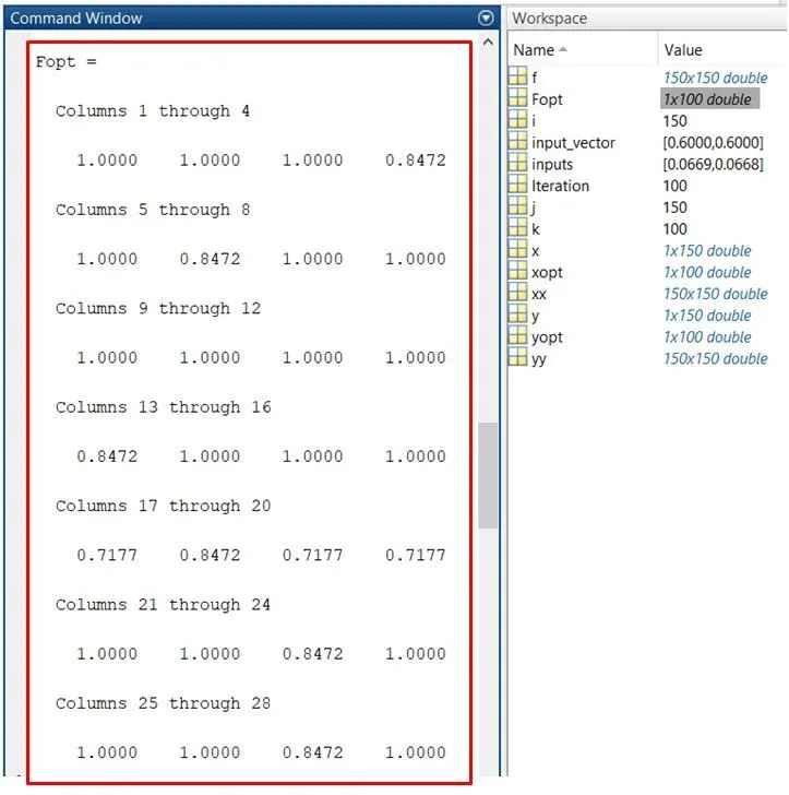
The global maxima deviation has been brought further low by constraining the fitness function with in the lower and the upper bounds.
Study-3:
Optimization with lower, upper bounds and population size
Code explanation:
- The search space, Iteration and input for the fitness function has been kept the same as like for the previous 2 studies.
- In the GA optimization function a for loop has been introduced for the number of iterations at which the GA function have to be operated.The GA function here used works based on the syntax x= ga(fun,nvars,A,b,Aeq,beq,lb,ub,nonlcon,options).By using the options featuring with in the function any desired input criteria can be add for requirement. Here we have used this to insert the population size in to the GA to get the very near optimum results.
The syntax has been modified the return the input and Fopt values as
[inputs,Fopt(k)]=ga(@stalagmite,2,[],[],[],[],[0;0],[0.6;0.6],[],[],options);
The linear equalities, inequalities and non linear constraints can be left empty for this syntax. The options calls the population size defined above in to the function to optimize for better results. - The result and global maximum deviation has been plotted in the same way as like in the previous cases.
Code:
clear all
close all
clc

%Study-3 Optimization with boundaries and population size
%Search space
x=linspace(0,0.6,150);
y=linspace(0,0.6,150);
Iteration=100;                                           %Number of iterations
[xx,yy]=meshgrid(x,y);

%Input for stalagmite function
for i=1:length(xx)
    for j=1:length(yy)
        input_vector(1)=xx(i,j);
        input_vector(2)=yy(i,j);
       f(i,j)=stalagmite(input_vector);
    end
end
f=-f;                                                    %To invert the surface plot


%Function optimization for the given iteration
options = optimoptions('ga');
options = optimoptions(options,'populationSize',250);    %To pass population size through GA syntax
tic
for k=1:Iteration
[inputs,Fopt(k)]=ga(@stalagmite,2,[],[],[],[],[0;0],[0.6;0.6],[],[],options);
xopt(k)=inputs(1);
yopt(k)=inputs(2);
end
toc
Fopt=-Fopt;                                                %To invert the optimum point

figure(1)
subplot(2,1,1)
surf(xx,yy,f)
title('Optimization with upper,lower bounds and population size')
xlabel('X-axis')
ylabel('Y-axis')
zlabel('Fopt')
shading interp
hold on
plot3(xopt,yopt,Fopt,'marker','o','markersize',5,'markerfacecolor','r')
subplot(2,1,2)
plot(Fopt)
title('Optimization with upper,lower bounds and population size')
xlabel('Iteration')
ylabel('Fopt')
Result: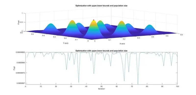
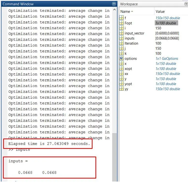
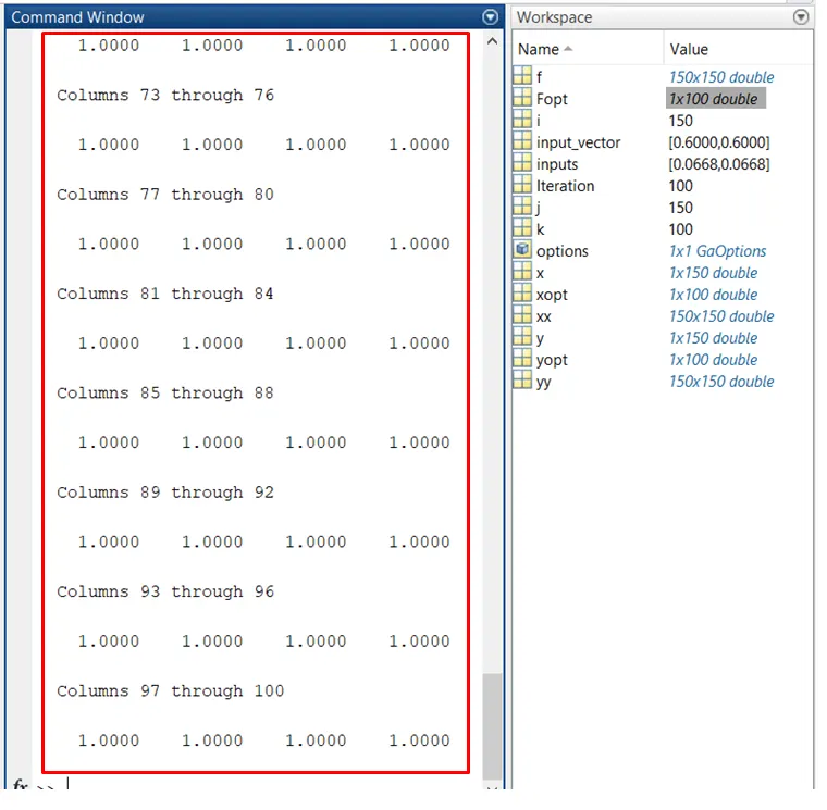
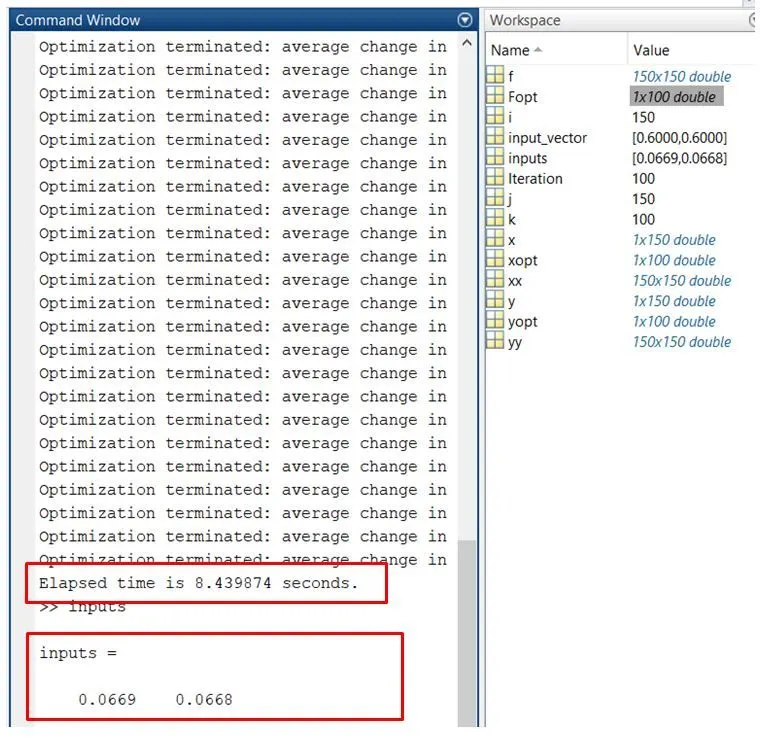
The global maxima has been optimized much better by assigning the population size to the function which gives additional constraints to the GA.
The Fopt deviation has been brought very much lower to yield more precise result.
Conclusion:
From the above study it has been found the results can be more accurate if the function was controlled in a better way by adding as much as constraints possible.
Errors thrown during coding:
There were no much errors faced during coding rather than few invalid expression errors which were correct by applying appropriate expressions like semi colon in the error lines.
References: