Project 1 - Parsing NASA thermodynamic data
NASA file parsing
Aim:
To understand the concept of file parsing to read the NASA’s thermodynamic data of different species and extract the coefficients to feed the polynomials in order to evaluate the thermodynamic properties of each species.
Objective:
To write Matlab code to perform the below tasks
- Open the ‘dat’ file and read the temperature data.
- Read and extract co-efficient and temperature range for each species.
- Calculate the molecular weight for each of the species.
- Calculate the specific heat(Cp), Enthalpy(H) and Entropy(S) for each species.
- Plot Specific heat, Enthalpy and Entropy for the temperature range from lower to higher.
- Save the figures of Specific heat, Enthalpy and Entropy for the temperature range with suitable name and pack the 3 figures for each species in a subfolders and dump it in a common folder.
Parsing:
Parsing is the process of breaking up a sentence or group of words into separate components, including the definition of each part's function or form. The technical definition implies the same concept.
To parse, in computer is where a string of data are separated into more easily processed components, which are analyzed for correct syntax and then attached to tags that define each component. The computer can then process each chunk of the components as desired by the user.
Parsing NASA thermodynamic file:
In this project the objective is to parse the given file in the name ‘THERMO.dat’ which is the thermodynamic file of NASA which contains the coefficient of polynomial for the set of species.
The file is in the format of containing the header information and the species block.The header information contains the global temperature range and comments.
The species block contains the species name, local temperature range and the polynomial coefficients, totally there are 53 species block available to read.
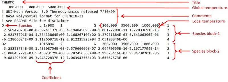
In order to find the Specific heat, Enthalpy and Entropy of each species the polynomial equation is given as,
`(Cp)/R=a1+a2T+a3T^2+a4T^3+a5T^4`
`H/(RT)=a1+ (a2T)/2+(a3T^2)/3+(a4T^3)/4+(a5T^4)/5+(a6)/T`
`S/R=a1lnT+a2T+(a3T^2)/2+(a4T^3)/3+(a5T^4)/4+a7`
Where, R=8.314 J/kg K (Universal gas constant) , T is temperature and a1 to a7 are coefficients.
In the species block we have a total of 14 coefficients where the first seven are for high temperature range and the second seven for low temperature range.So the above equation can be used for high temperature range, and for low temperature range the equation can be written as,
`(Cp)/R=a8+a9T+a10T^2+a11T^3+a12T^4`
`H/(RT)=a8+ (a9T)/2+(a10T^2)/3+(a11T^3)/4+(a12T^4)/5+(a13)/T`
`S/R=a8lnT+a9T+(a10T^2)/2+(a11T^3)/3+(a12T^4)/4+a14`
Here a8 to a14 represent the coefficients for low temperature range.Each of the species block contains the respective temperature range in the sequence of local low temperature, local high temperature and local mid temperature which should be substituted in to the above equation.On passing the temperature and the coefficient data in to the above equations we can calculate the specific heat, enthalpy and entropy for each of the species.Along with calculating the specific heat, enthalpy and entropy the molecular weight of the species have to be calculated by reading the species element.
Code:
clear all
close all
clc

%Opening the thermo data
data=fopen('THERMO.dat','r');

%Reading header information
Title=fgetl(data);
Global_temp_range=fscanf(data,'%f');
Global_low_Temperature=Global_temp_range(1);
Global_mid_Temperature=Global_temp_range(2);
Global_high_Temperature=Global_temp_range(3);

%Reading comments
for comment=1:3
comment=fgetl(data);
end

%Reading species block
for i=1:53
get_line1=fgetl(data);
line_length=length(get_line1);
line_1=strsplit(get_line1,' ');
species=line_1{1};
y=length(line_1);

%Reading local temperature
Local_low_temperature=str2double(line_1{y-3});
Local_mid_temperature=str2double(line_1{y-1});
Local_high_temperature=str2double(line_1{y-2});

%Reading species block line-2
get_line2=fgetl(data);
line_2=strfind(get_line2,'E');
a1=get_line2(1:line_2(1)+3);
a1=str2double(a1);
a2=get_line2(line_2(1)+4:line_2(2)+3);
a2=str2double(a2);
a3=get_line2(line_2(2)+4:line_2(3)+3);
a3=str2double(a3);
a4=get_line2(line_2(3)+4:line_2(4)+3);
a4=str2double(a4);
a5=get_line2(line_2(4)+4:line_2(5)+3);
a5=str2double(a5);

%Reading species block line-3
get_line3=fgetl(data);
line_3=strfind(get_line3,'E');
a6=get_line3(1:line_3(1)+3);
a6=str2double(a6);
a7=get_line3(line_3(1)+4:line_3(2)+3);
a7=str2double(a7);
a8=get_line3(line_3(2)+4:line_3(3)+3);
a8=str2double(a8);
a9=get_line3(line_3(3)+4:line_3(4)+3);
a9=str2double(a9);
a10=get_line3(line_3(4)+4:line_3(5)+3);
a10=str2double(a10);

%Reading species block line-4
get_line4=fgetl(data);
line_4=strfind(get_line4,'E');
a11=get_line4(1:line_4(1)+3);
a11=str2double(a11);
a12=get_line4(line_4(1)+4:line_4(2)+3);
a12=str2double(a12);
a13=get_line4(line_4(2)+4:line_4(3)+3);
a13=str2double(a13);
a14=get_line4(line_4(3)+4:line_4(4)+3);
a14=str2double(a14);

%Calculating Molecular weight
Element=['O', 'H', 'C', 'N', 'A', 'S'];                          %Elements of species
Atomic_weight=[15.999, 1.0080, 12.011, 14.007, 39.9, 32.07];     %Atomic weight of the elements
Molecular_weight=0;

for j=1:length(species)
    for k=1:length(Element)
        if strcmp(species(j),Element(k))
            Molecular_weight=Atomic_weight(k)+Molecular_weight;
            qty=k;
        end
    end
    number=str2double(species(j));

    %Calculating molecular weight
    if number>1
        Molecular_weight=Molecular_weight+Atomic_weight(qty)*(number-1);
    end
end

%Printing molecular weight for each species
Mole_statement='Molecular weight of %s is %f g/mol\n';
    fprintf(Mole_statement,species,Molecular_weight);

%Calculating Specific heat(Cp), Enthalpy(H) and Entropy(S)
R=8.314;

   Temperature=linspace(Local_low_temperature,Local_high_temperature,1000);              %Local temperature range
   for t=1:length(Temperature)
      if Temperature(t)>=Local_mid_temperature
          Cp(t)=(a1+a2*Temperature(t)+a3*Temperature(t)^2+a4*Temperature(t)^3+a5*Temperature(t)^4)*R;
           H(t)=(a1+a2*Temperature(t)/2+a3*(Temperature(t)^2)/3+a4*(Temperature(t)^3)/4+a5*(Temperature(t)^4)/5+a6/Temperature(t))*R*Temperature(t);
           S(t)=(a1*log(Temperature(t))+a2*Temperature(t)+a3*(Temperature(t)^2)/2+a4*(Temperature(t)^3)/3+a5*(Temperature(t)^4)/4+a7)*R;
      else
          Cp(t)=(a8+a9*Temperature(t)+a10*Temperature(t)^2+a11*Temperature(t)^3+a12*Temperature(t)^4)*R;
           H(t)=(a8+a9*Temperature(t)/2+a10*(Temperature(t)^2)/3+a11*(Temperature(t)^3)/4+a12*(Temperature(t)^4)/5+a13/Temperature(t))*R*Temperature(t);
           S(t)=(a8*log(Temperature(t))+a9*Temperature(t)+a10*(Temperature(t)^2)/2+a11*(Temperature(t)^3)/3+a12*(Temperature(t)^4)/4+a14)*R;
      end

   end

   %Plotting output
   figure(1)
   plot(Temperature,Cp,'linewidth',3,'color','blue')
   xlabel('Temperature(K)')
   ylabel('Specific heat(J/kg·K)')
   title({"Species-"+species;'Temperature vs Specific heat'})

   figure(2)
   plot(Temperature,H,'linewidth',3,'color','magenta')
   xlabel('Temperature(K)')
   ylabel('Enthalpy( kJ/mol)')
   title({"Species-"+species;'Temperature vs Enthalpy'})

   figure(3)
   plot(Temperature,S,'linewidth',3,'color','cyan')
   xlabel('Temperature(K)')
   ylabel('Entropy(kJ/K)')
   title({"Species-"+species;'Temperature vs Entropy'})

   %Saving output
   if i==1
   main_directory=pwd;
   mkdir('Species data');
   directory_1=([pwd,'\species data\']);
   cd(directory_1);
   mkdir(species);
   directory_2=([pwd,'\',species]);
   cd(directory_2);
   saveas(figure(1),'Specific heat.jpg');
   saveas(figure(2),'Enthalpy.jpg');
   saveas(figure(3),'Entropy.jpg') ;
   cd(main_directory);
   else
   directory_1=([pwd,'\species data\']);
   cd(directory_1);
   mkdir(species);
   directory_2=([pwd,'\',species]);
   cd(directory_2);
   saveas(figure(1),'Specific heat.jpg');
   saveas(figure(2),'Enthalpy.jpg');
   saveas(figure(3),'Entropy.jpg');
   cd(main_directory);
   end

end
fclose(data);
Code explanation:
- Open the ‘THERMO.dat’ file using the command ‘fopen’ and read using the command ‘r’ and store it in the array named ‘data’, this gives a positive value to the array once opened.
- Read the title of the file using the command ‘fgetl’ from the array called ‘data’ and store it in a new array named ‘Title’.
- Read the global temperature range for low medium and high using ‘fscanf’ command for floating point numbers and store it in a variable named ‘Global_temp_range’.
All the 3 temperature will be stored in 3 cells, and the 3 values are low medium and high temperature. - Read the comment lines by using ‘fgetl’ command for 3 times for 3 lines using ‘for’ loop and store it in the array named ‘comment’.
- Reading coefficients of each species
- A ‘for’ loop has been created to read the coefficients and local temperature range for 53 species blocks.
- In side of the ‘for’ loop the reading process continues using ‘fgetl’ command to read the first line and store it in an array named ‘get_line1’
- The first line contains the information such as species name, local temperature range, etc. here our intention is to store the species name and temperature range only. These elements have spaces in common which separates each other.
This line can be fragmented for the number of elements with space separations, this can be done using ‘strsplit’ command. This will identify the strings which the user desires and split the lines for the number of times the assigned strings are found in the line. Here the string we assigning is the space. Using the ‘strsplit’ command over the array ‘get_line1’ by identifying the space the line got fragmented and stored in cells of the array named ‘line_1’. - The species name is the first cell of line_1 which is stored in an array called ‘species’.
- Find the length of the line and store it in an array named ‘y’. this will be used to store the local temperature values.
- The local, low medium and high temperature can be read by ranging the location where the values actually are in the first line. As we know the array ‘y’ stores the length of the line, there by subtracting the length by the position of the particular character counting from the rear of the line. The temperature got read will be in the format of string which have to be converted in to double precision value by using the command ‘str2double’. With this algorithm all the 3 temperature can be respectively stored as low, mid and high temperature in appropriate array.
- The next step is to find the coefficients from a1 to a14 for low to high temperature. This can be done by using the ‘fgetl’ command over the array ‘data’ and stored it in another array named ‘get_line2’.
- To read the coefficient the logic used is to position a point from which the range forward and backward can be the coefficient. To fix the position the identified=r chosen was the character ‘E’ which denotes the exponent. 2 position after the character ‘E’ is the exponential value, the rest of the elements before the character ‘E’ is the coefficient number.
The character ‘E’ was identified using the comment ‘strfind’. This command will spot the user defined character (in our case ‘E’ is the string we intend to find).
store the position of ‘E’ through out the line in an array named ‘line_2’ each of the position will be stored in separate cells. - Each coefficient was stored in their respective array (say a1,a2,a3,etc, up to a14)
using the ‘fgetl’ command over the range in front of and after the character ‘E’.
all the coefficients are in the string format was converted in to double precision values using ‘str2double’ command. - The above step was repeated to read the line-3 and 4.
- Calculating molecular weight if the species
- Store the total number of elements represented though out the thermodynamic file in a sequence in a vector array named ‘Elements’. All those elements are in separate cells.
- Store the atomic weight of each of the elements in a vector array names ‘Atomic_weight’ in the same sequence like the ‘Elements’.
- Initialize the molecular weight as 0 in an array named ‘Molecular_weight’, this will be retrieved back for calculating the molar mass.
- Initialize a ‘for’ loop for the length of the species characters.
- Inside of the ‘for’ loop initialize the nested ‘for’ loop for the length of the elements array.
- The logic is to compare the species character against the character of the elements, if the result comes true the correct species is spotted for which the atomic weight can be assigned.
- The comparison was done using the ‘if’ statement and the ‘strcmp’ command to compare the element of ‘j’ and ‘k’.
- If the comparison result is true the molecular weight will be calculated by adding up the atomic weight of each species. If the result is false it will jump over the next cell of the ‘Element’ vector array.
- If there any number present in the species to sum the species times the number which need to be identified, that was done using the ‘str2double’ command over the element of ‘j’ and stored in an array named ‘number’.
- An ‘if’ statement was used to find if the number greater than 1, if so then the molecular weight calculation formula has to be used is the sum of molecular weight times the atomic weight times the number which is greater than 1. This process repeat for the length of the species to calculate the molecular weight.
- After the end of the molecular weight calculation loop the molecular weight was printed in command window using ‘fprintf’ command.
- Calculating Specific heat (Cp), Enthalpy (H) and Entropy(S)
- Assigned the universal gas constant to an array named ‘R’ which is required to calculate specific heat, enthalpy and entropy.
- Assigned the temperature range from low to high with 1000 units using ‘linspace’ command from the input read and stored as low and high temperatures.
- The temperature range was stored as a vector array in the name ‘Temperature’.
- Initialized a ‘for’ loop for the length of the temperature range, for each temperature the Cp, H and S will be calculated.
- The Cp, H and S coefficients varies for low and high temperature range. Where a1 to a7 is high temperature range and a8 to a14 is low temperature range.
- The low and high temperature ranges are categorized using the ‘if’ statement.
where if the temperature is greater than or equal to the mid temperature value stored in the array ‘Local_mid_temperature’ the high temperature coefficients a1 to a7 will be assigned to the Cp, H and S formula, else the low temperature coefficients a8 to a14 will be assigned to the Cp, H and S formula. - The loop ends after reading the 1000 units of temperature range.
- Plotting thermodynamic data
- 3 figures has been plotted for Specific heat, Enthalpy and Entropy for Temperature using ‘plot’ command.
- Figure-1 Temperature vs Specific heat
- Figure-2 Temperature vs Enthalpy
- Figure-3 Temperature vs Entropy
- Saving output
- Our intention is to store the above 3 figures in to a folder in the name of the species for which the Cp, Enthalpy and Entropy was calculated in a separate main folder. With this process all the 159 figures for 53 species have to get packed in to 53 folders for respective species.
- Store the current working directory path in an array named ‘main_directory’ using the ‘pwd’command, which gets the path of current working directory.
- Create a new folder in the name ‘Species data’ using ‘mkdir’ command inside the main folder.
- Construct a path by adding ‘\species\’ to the current working directory (pwd) and store it in an array named ‘directory_1’
- Change the current working directory to ‘diectory_1’ using the change directory ‘cd’ command.
- Create another subfolder in the name of the current species we are reading to store the temperature figures using the command ‘mkdir(species)’
- Add the new folder path to the up one level folder by adding it to the path and store it as ‘directory_2’
- Change the current working directory to ‘diectory_2’ using the change directory ‘cd’ command.
- Use the ‘saveus’ command to save figure 1,2 and 3 with the desired file name
- Change the current directory to main directory again using the command ‘cd’
- An ‘if’ statement was used to create the subfolder where are the species data are stored while reading the first species when the result of the ‘if’ statement is true (if==1). Else all other folders in the name of respective species will be stored directly to the first created level-2 folder.
- The above process repeats for 53 time in the ‘for’ loop to read all the 53 species blocks, Once all the species data are extracted and output computed and stored the file will be closed using ‘fclose’ command which returns the answer as ‘0’ if the file was closed.
Output:
- Molecular weight for each species from command window
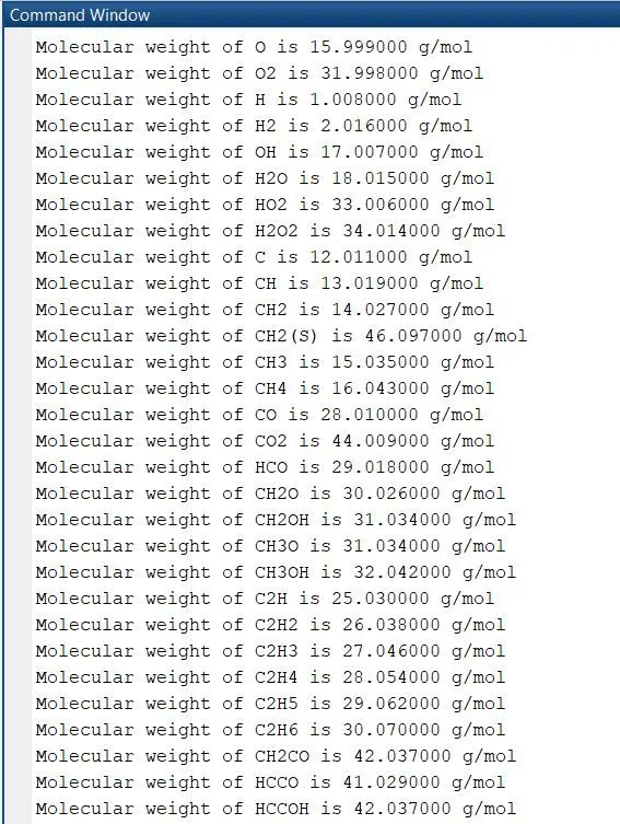
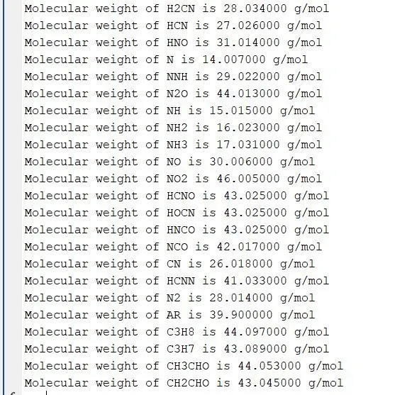
- Screenshot of the window where all the folders are saved
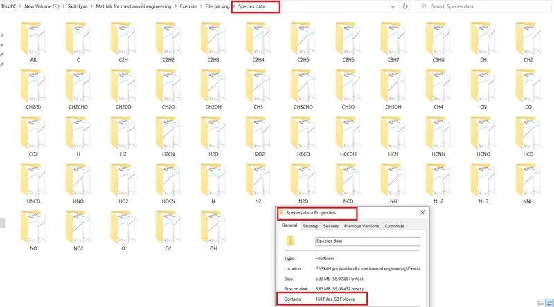
-
Plots for O2, N2 and CO2 species
- O2
Temperature vs Specific heat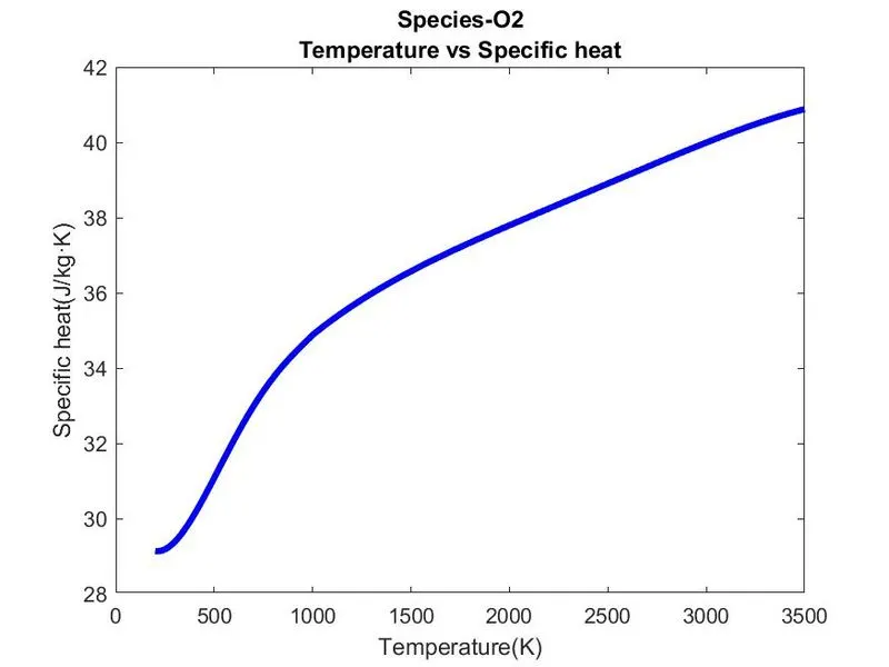
Temperature vs Enthalpy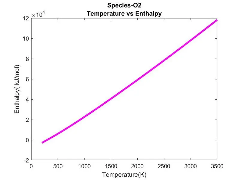
Temperature vs Entropy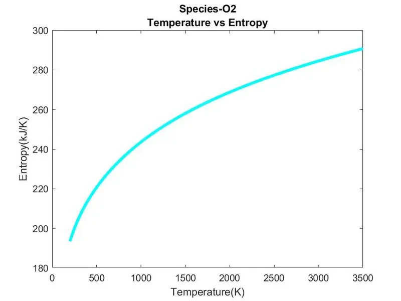
- N2
Temperature vs Specific heat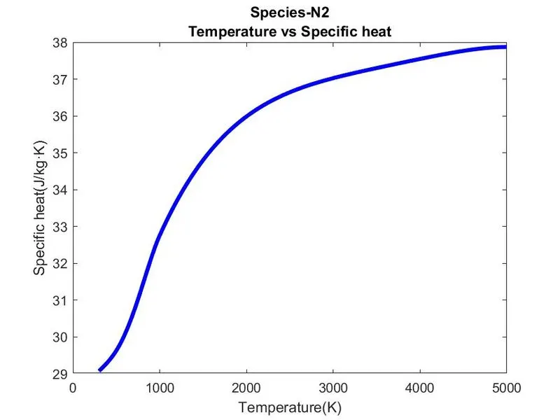
Temperature vs Enthalpy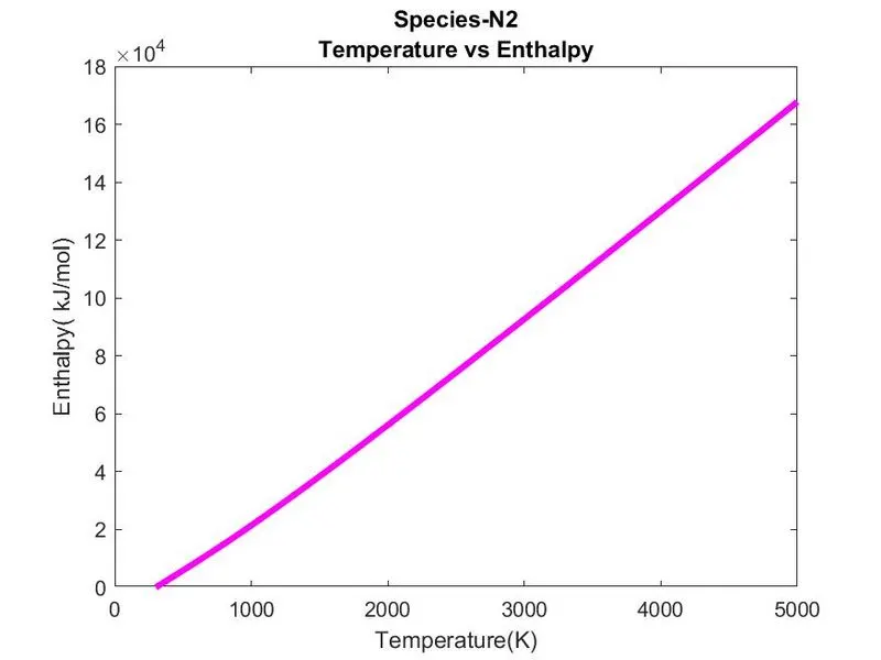
Temperature vs Entropy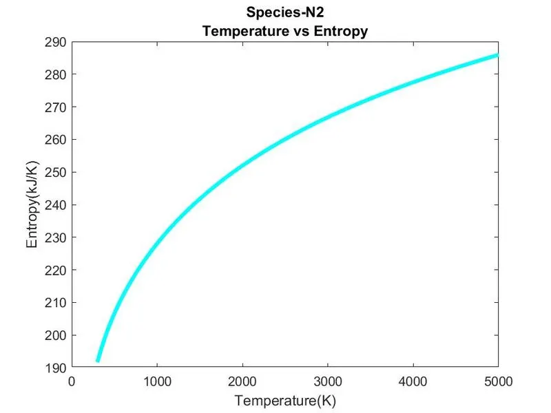
- CO2
Temperature vs Specific heat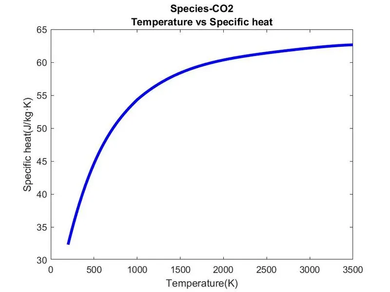
Temperature vs Enthalpy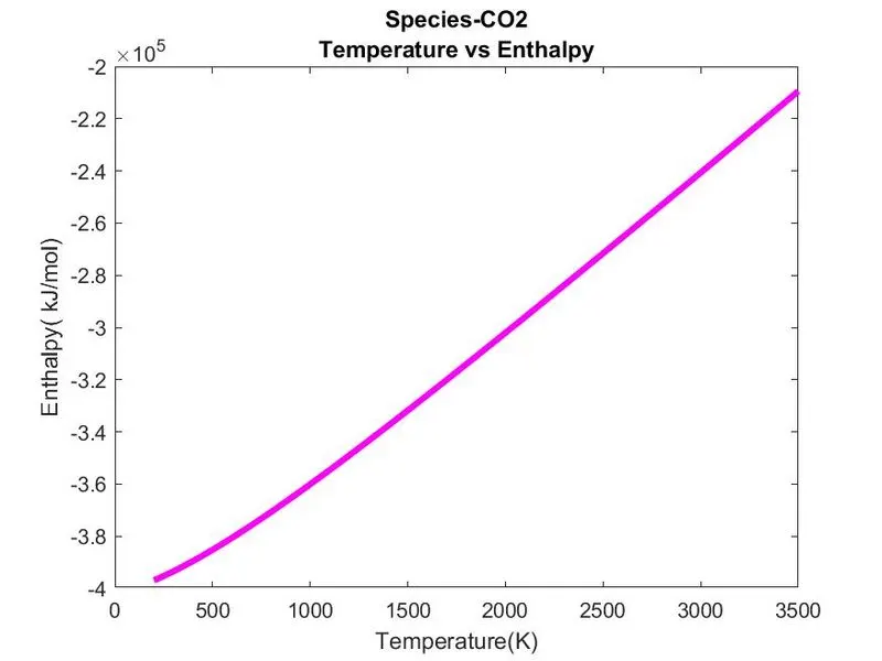
Temperature vs Entropy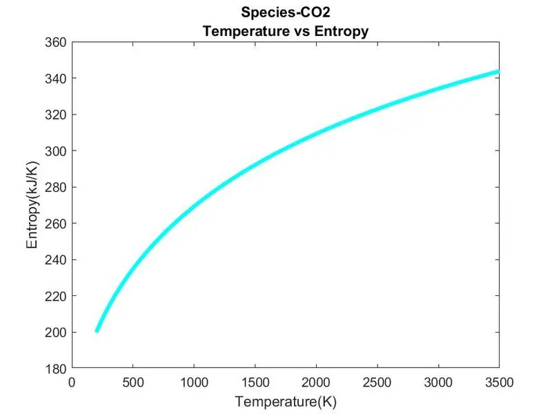
- O2
Errors thrown during coding:
There were no much errors faced during coding rather than few invalid expression and minor logic errors which were correct by applying appropriate expressions and correcting the logic.
References:
https://in.mathworks.com/help/matlab/ref/strcmp.html?searchHighlight=strcmp&s_tid=srchtitle
https://in.mathworks.com/help/matlab/ref/mkdir.html#d122e835531
https://in.mathworks.com/help/matlab/ref/pwd.html#d122e1031786
https://in.mathworks.com/help/matlab/ref/cd.html#d122e140483
https://in.mathworks.com/help/matlab/ref/saveas.html?searchHighlight=saveas&s_tid=srchtitle
https://pubchem.ncbi.nlm.nih.gov/periodic-table