Week 3 - Solving second order ODEs

Solving second order ODE for Simple pendulum using Matlab

Aim:

To simulate the motion of the simple pendulum under 2^nd order ordinary differential equation and to plot the behavior of angular velocity and displacement at the given time.

Theory of Simple pendulum:

A simple pendulum is a mechanical system where a massive bob is suspended to a rigid support with a help of a string of negligible mass which makes the bob to get pivoted to the fixed point support.

The simple pendulum would be set to oscillation under the influence of gravity and friction coefficient, in an ideal pendulum the co-efficient of would be considered as zero.

The simple pendulum oscillates to the time period ‘T’ depending up on the mass of the pendulum ‘m’, length of string ‘l’ ,the strength of the gravity and the damping co-efficient.

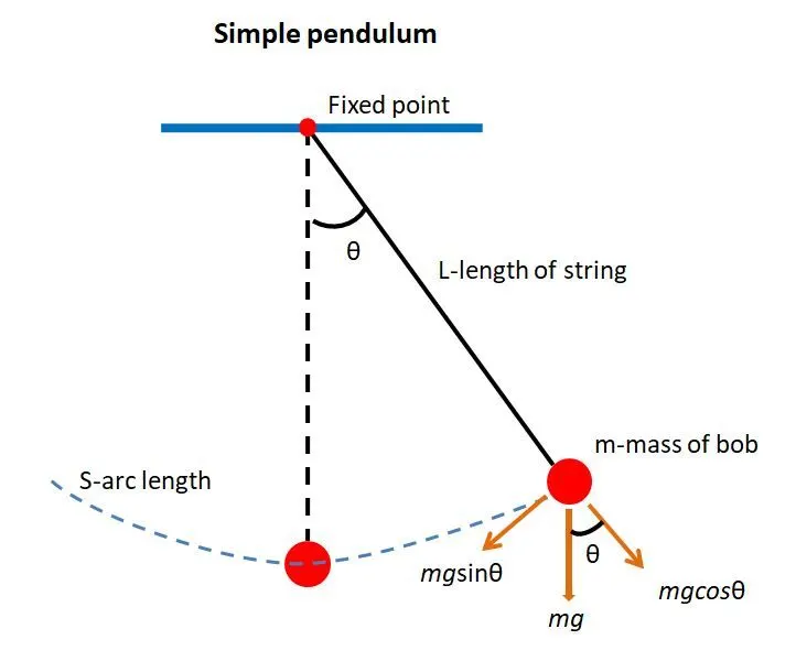
The behavior and motion of a practical pendulum under the influencing factors can be determined by solving the 2^nd order ordinary differential equation with the function of time as below.

`(d^2 θ)/(dt^2 )+b/m dθ/dt+g/L sin⁡θ=0`

From the above equation,

g = gravity in m/s2,

L = length of the pendulum in m,

m = mass of the ball in kg,

b=damping coefficient.

Objective:

• Write a Matlab main program to determine the angular velocity and angular displacement at the give time period
• Write a Matlab ODE function to solve the second order ODE
• Plot the graph for the behavior of angular velocity and angular displacement
• Simulate the motion of the pendulum with the obtained ODE results.

Given data:

L=1 M

m=1 kg,

b=0.05.

g=9.81 m/s^2

Time span=20sec

Angular displacement=0

Angular velocity=3red/sec

Code explanation:

Matlab Main program:

The main program start with the consist of the given input data

l=1, Length of string (meter),

m=1, Mass of the bob (kg),

b=0.05, Damping co-efficient

g=9.81, Acceleration due to gravity m/s^2

Initial condition

Angular displacement =0

Angular velocity=3 rad/sec

The above 2 input will be stored in an array named ‘theta_0’

Time span=20secs and will be stored as ‘t_span’

As we know that the change in the angular displacement and velocity is a function of time,

The ODE have to be solved by creating and calling a function which computes the change in angular displacement and angular velocity as the function of time.

The ode solver ‘ode45’ has been used to solve the ODE.

Here we are integrating the ODE function with the given input time span and the initial conditions of angular displacement and velocity with the help of the ODE solver command.

The input parameters (Time span and initial conditions) will be included with the ode45 command which is basically executing ‘θ’ as a function of time ‘t’.

The ode45 calls the function which computes the angular displacement and velocity for each values when being integrated with the initial conditions for the given time period.

The output, change in angular displacement and angular velocity will be stored in an array called ‘result’ for the time period of 20sec with 500 values at the first and second column respectively.

Plotting amplitude vs time

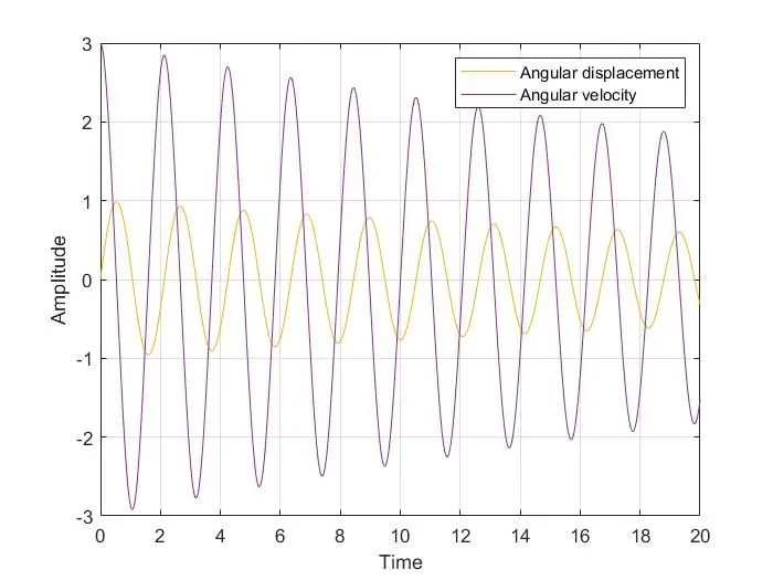
The behavior of the amplitude of the simple pendulum with respect to time has been plotted graphically with the value stored in the array ‘result’. Where column-1 is angular displacement and column-2 is angular velocity.

Pendulum motion simulation.

The motion of the simple pendulum has been simulated as an animation.

We know that for each value of the angular displacement the pendulum oscillates to and fro.

The displacement values stored in the column-1 of the result array can be retrieved to calculate the position ‘x’ and ‘y’ of the bob .

The relation to determine the position of the bob can be written as

X=L*Sinθ (for X co ordinate)

Y=L*Cosθ (for Y co ordinate)

To pick the value of angular displacement (θ) a ‘for’ loop have to be executed every time for the length of the first column in the result array.

Each time the ‘for’ loop executes it will compute the value for x and y co ordinates and stores the value in the array ‘x1’ and ‘y1’.

For 500 units for the given time period it will executes the ‘for’ loop for 500 times and stores the values to the array x1 and y1 which can be plotted to simulate the position of the string and the bob using ‘plot’ command.

Matlab function program:

To execute the main program the ode45 command need to call the function to determine the value of θ1 and θ2 which was done by creating a function under function definition ‘ode_function’

This ode function takes the input values of l,b,m and g from the main program and executes the governing equation.

For 2^nd order ODE the equation must need to be split in to 2 first order ODEs and the results will be stored as θ1 and θ2 respectively is the angular displacement and angular velocity.

The breaking down of the 2^nd order ODE is as below.

Breaking down of 2^nd order ODE in to first order ODEs.

As the ODE is of the form 2^nd order so this needs to be broken down in to 1^st order ODEs as below.

Governing equation,

`(d^2 θ)/(dt^2 )+b/m dθ/dt+g/L sinθ=0`

Breaking down the 2^nd order ODE in to 1^st order ODEs as,

`dθ/dt=(dθ_1)/dt=θ_2 →equ(1)`

From`equ(1)`

`(d^2 θ)/(dt^2 )=(d^2 θ_1)/(dt^2 )=d/dt ((dθ_1)/dt)=d/dt (θ_2 )`

From equ (1) the general equ can be written as,

`(d^2 θ_1)/(dt^2 )+b/m (dθ_1)/dt+g/L sinθ_1=0`

The above equation can also be written as,

`d/dt (θ_2 )+b/m θ_2+g/L sinθ_1=0 →equ(2)`

From equation (1) and (2)

`(dθ_1)/dt=θ_2`

`(dθ_2)/dt= - b/m θ_2- g/L sinθ_1`

which implies,

`d/dt [█(θ_1@θ_2 )]=[█(θ_2@- b/m θ_2- g/L sinθ_1 )]`

Where, θ1 is angular displacement and θ2 is angular velocity

The computed values of θ1 and θ2 has been stored in the array ‘dtheta1_dt and dtheta2_dt’ respectively.

The values of dtheta1_dt and dtheta2_dthas been collectively stored in an array of matrix form called ‘dtheta_dt’ in column-1 and column-2 respectively.

Code used:

Main program

clear all
close all
clc

%Simple pendulum simulation using 2nd order ordinary differential equation
%Input parameters
l=1; %Length of string (meter),
m=1; %Mass of the bob (kg),
b=0.05; %damping co-efficient
g=9.81; %Acc due to gravity m/s^2

%Initial condition
theta_0=[0;3]; %Where initial angular displacement is 0rad and angular velocity at initial condition is 3rad/sec
t_span=linspace(0,20,500); %Time span is 20sec

%ODE solver calls the funtion for the ODE and stores the result in the
%array named 'result' where column-1 is angular displacement and column-2 is angular velocity
[t, result]=ode45(@(t,theta)ode_function(t,theta,b,l,m,g),t_span,theta_0);

%Plotting values
figure(1)
plot(t,result(:,1));
hold on
plot(t,result(:,2));
xlabel('Time')
ylabel('Amplitude')
legend([plot(t,result(:,1)) plot(t,result(:,2))],{'Angular displacement','Angular velocity'})
grid on

%Program to determin the position of bob with respect to the anguler position of the pendulum

%Fixed point where the pendulum string is hinged
x0=0;
y0=0;

%Angular displacement is the rate of change of the angular position which
%can be obtained from the theta_1 of the result from ODE function stored in
%the 1st column of the array 'result'
angular_displacement=result(:,1);
ct=1;
figure(2)
for i=1:length(angular_displacement)    

x1=-l*sin(angular_displacement(i))
y1=-l*cos(angular_displacement(i))

%Plotting the position of bob and string
plot([-0.5 0.5],[0 0],'linewidth',4,'color','k')
hold on
plot([x0,x1],[y0,y1],'color','k','linewidth',1);
hold on
plot(x1,y1,'-o','color','r','markerfacecolor','r','linewidth',20);
hold off
axis([-1 1 -2 1])
xlabel('X-axis')
ylabel('Y-axis')
text(-0.7,0.5, 'Simple pendulum motion animation','fontsize',15)
M(ct)=getframe(gcf);
ct=ct+1;

end

%Creating video file
movie(M);
output=VideoWriter('Simple pendulum 2nd order ODE.avi','uncompressed avi')
open(output)
writeVideo(output,M)
close(output)

Function program

%The function definition for the 2 order ODE is as below
function [dtheta_dt]= ode_function(t,theta,b,l,m,g)
theta1=theta(1);
theta2=theta(2);

dtheta1_dt=theta2;%Rate of change of angular displacement
dtheta2_dt=-(b/m)*theta2-(g/l)*sin(theta1);%Rate of change of angular velocity

dtheta_dt=[dtheta1_dt;dtheta2_dt];

end

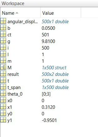
Work space

Result:

Amplitude VS Time

Animation simulation:

https://youtu.be/Gr1xrDb8zrk

Errors thrown:

Error-1

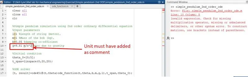
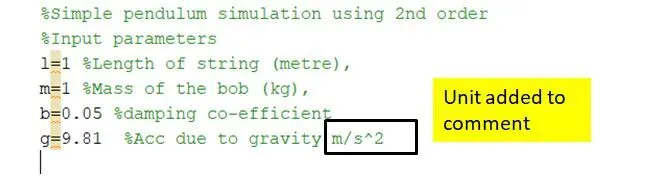
This error was resolved by moving the unit in to comments

Error-2

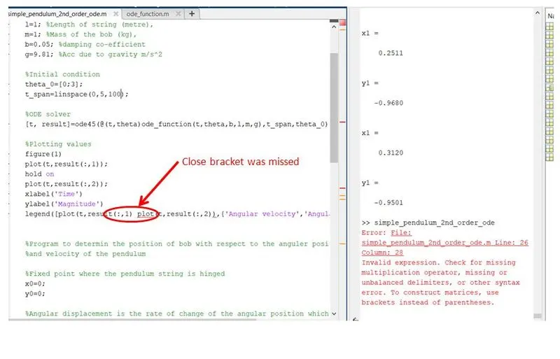
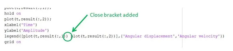
This error was resolved by adding the missing close bracket