Week 4 - Genetic Algorithm

MATLAB program to optimize the stalagmite function and finding the global maxima of the function

Aim:

• Explain the concept of genetic algorithm and syntax for ga in MATLAB.
• Write s a MATLAB code to optimize stalagmite function using genetic algorithm and find the maximum of the function.

THEORY:

GENETIC ALGORITM:

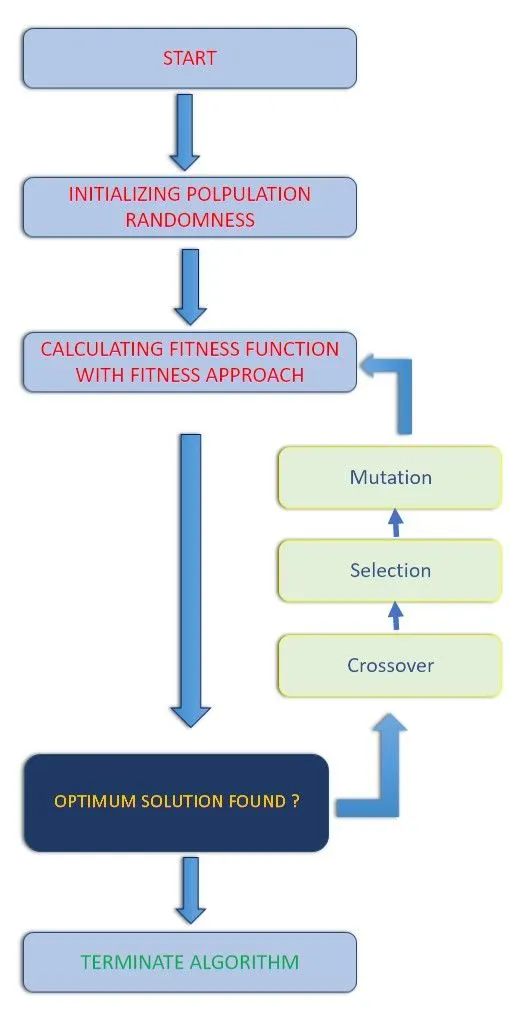
A genetic algorithm is a search algorithm that is inspired by Charles Darwin’s theory of natural evolution. This algorithm reflects the process of natural selection where the fittest individuals are selected for reproduction in order to produce offspring of the next generation.

in other words : A genetic algorithm (GA) is a method for solving both constrained and unconstrained optimization problems based on a natural selection process that mimics biological evolution. The algorithm repeatedly modius a population of individual solutions. At each step, the genetic algorithm randomly selects individuals from the current population and uses them as parents to produce the children for the next generation. Over successive generations, the population "evolves" toward an optimal solution.

\

WORKING OF GENATIC ALGORITHM

Genatic algorithm optimisation starts with population initialization

Population is the number of sample data points taken to perform the genetic algorithm operation.

These sample data points undergoes the following three steps:

• Crossover:

It is the process of taking two parents' solutions and producing the child from them.

• Selection:

In this, the parents are selected from the sample data points, the main objective of the selection process is to select the highly fit individuals

• Mutation:

Mutation is carried out to maintain the genetic diversity from one generation of a population of chromosomes to the next.

Fitness function:

Fitness function takes the solution as input and produces the suitability of the solution as the output. This evaluates how close the solution is to the optimal solution of the desired problem.

Syntax for Genetic Algorithm:

(refrence form Matlab help center)

%defining the function name and input values required to evaluate
function s_r= stalagmite_fn(input) % fn stalagmite_fn is called with input as input variable 
x=input(1); %x stores the 1st value in matix of input variable
y=input(2); %y stores the 2nd value in matix of input variable
f1x=[sin(5.1*pi*x+0.5)]^6; %f1 is evaluatd
f1y=[sin(5.1*pi*y+0.5)]^6; %f2 is evaluated
f2x=exp((-4*log(2)*((x-0.0667)^2)/0.64)); %f3 is evaluated
f2y=exp((-4*log(2)*((y-0.0667)^2)/0.64)); %f4 is evaluated
% finaly the value of f is evaluated using f1*f2*f3*f4 
s_r=-(f1x*f1y*f2x*f2y); % evaluated f value is passed to s_r that is returned by the function stalagmite_fn
end

To define the stalagmite function:

1.define the name as stalagmite_fn and use it by passing 'inputs' variable as input for the function

2. it returns the the value in s_r.

3. put the 1st value in input as x and second value as y.

4.with thw use of formula for the function define f1x,f2x,f1yf2y.

5.return the s_r values as negative of the product of f1x,f2x,f1y&f2y;

• get_stalagmite function:

to calculate the result from the stalagmite function for the grid.

%function to get the ploting values of stalagmite function at diffrent(x,y) co-ordinate values
function f=get_stalegmite(x,y) % function get_stalagmite is passed with limiting values for plot (x,y)
%creating a 2d mesh
[xx yy]=meshgrid(x,y);% generate the grid of x and y values (area =x*y)
%evaluating stalagmite fn
%nested loop to evaluate values of stalagmite function for generated grid values 
for i=1:length(xx)% 1st loop to get x values
 for j=1:length(yy)% 2nd loop to get y values
     %extracting input values form meshgrid 
    input(1)=xx(i,j);%x is stored as xx(i,j)
    input(2)=yy(i,j);%y is stored as yy(i,j)
    f(i,j)=stalagmite_fn(input);%stalagmite function is evaluated for the input value and result is stored in f for co-ordinate (i,j)
 end 
end
end

To define the get_stalagmite:

1.pass the x and y values defined for the result space in get_stalagmite function.

2. f is the value returned by the function.

3.create a grid of values using meshgrid from x and y values.

4.use nested for loop to get the value of stalagmite function at each point on grid of x and y values.

5. save the result in a variable x of 2 dimentional matrix with its co-ordinates.

• STATICAL BIHAVIOUR

To study the behaviour of the genetic algorithm without applying any condition to the optimisation process.

Explanation:

1. Program sarts with clear all close all clc to clear and close the files opened in command window.
2. defining the research space for the stalagmite function using linespace command for x and y values.
3. then the function get_stalagmite is called to calculate the function value over the defined x-y grid.
4. to find the maximum for the function the function is reversed with a negative sign.
5. tic and toc command is used to get the study time taken for the ga to run.
6. for loop is used to run the ga for 50 times using the value in num_case variable defined before the loop .
7. ga is called and stalagmite_fn is optimised for the loop and optimum value with their co-ordinate is stored.
8. ga is defined with function name and no of variables
9. for ploting the output results of the stalagmite_function and and optimised values through ga.
10. figure command is used to plot diffrent graphs on same figure window.
11. for the 1st graph using plot command the stalagimte function is ploted and the optimised value is shown.
12. for the 2nd graph plot command is used to plot the optimum value with its corosponding itrration number.
13. xlabel and ylabel is used to define axies names.

PROGRAM

clear all
close all
clc

%defining the research space
x=linspace(0,0.6,150);%150 values in 0 to 0.6 are stored in x
y=linspace(0,0.6,150);%150 values in 0 to 0.6 are stored in y

%num_case is defind to run the ga for the function in loop
num_case=50;%num_case is initialised to 50

%get_stalagmite function is called to callculate the stalagmite function value for the x and y mesh grid values.
F=get_stalegmite(x,y);%F is storing the results from the get_stalagmite function

% TO GET THE MAXIMUM OF THE FUNCTION
%this is done to reverse the stalagmite function results into stalagtite function so that we can find the maximum of the function
f=-F;%f is given the negative values of F 

%tic and tac command is used to get the time needed to solve for theresult
tic

%for loop is used to run the genetic alogorithm for several times to get the optomised result
for i=1:num_case % in this case this is made to run 50 times
    %genetic algorithm is used to find the minimum of the function
    %fopt and its co_ordinates aare returned as results
    [inputs,fopt(i)]=ga(@stalagmite_fn,2)% funtion is passed through ga 
    xopt(i)=inputs(1);%1st result of input is the x- co_ordinate of that fopt value.
    yopt(i)=inputs(2);%2nd result of input is the y- co_ordinate of that fopt value.
end

%FOR MAXIMUM OF THE FUNCTION
%the optimum varules from the results of ga give minimum value so reverse
%the results with a negative sign
fopt=-fopt%-tive sign is used to find maximum of the function


% timer for the study is stoprd with toc comand
study_time=toc%study_time stored the time value for the ga to solve


%figure window is called with figure comand
figure(1) %for the first figure

%two plots are made in the same figure windom to explain the result
%subplot commnd is used
subplot(2,1,1)%for the 1st subplot
hold on%hold on comand is used to hold the results
surfc(x,y,f)%surface command is used to plot the graph with x values , y values and its corosponding values
shading interp %shape interp is used to get smoth surface with grid lines
xlabel("X axies")% x is labled as x axies
ylabel("Y axies")% y is labled as y axies
zlabel("Z axies")% z is labled as z axies

%now plot command is used to plot the fopt values for the maximum of the function
plot3(xopt,yopt,fopt,'marker','o','markersize',5,'markerfacecolor','r')

%using subplot command to open the second plot for the same figure
subplot(2,1,2)
plot(fopt)%polt comand is used to plot the fopt value 
xlabel("ittration")%% x is labled as ittration
ylabel("maximum_of_fn")% y is labled as maximum_of_fn

RESULTS :

the time to obtain the result was least but the randomness in the result is too much and the optimised result is also beyond the research space.

Statical Behaviour TOP View		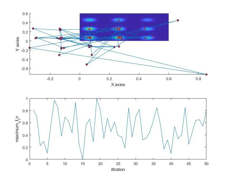the graph show a lot of variation durring the ittration process
Statical Behaviour X-Z View		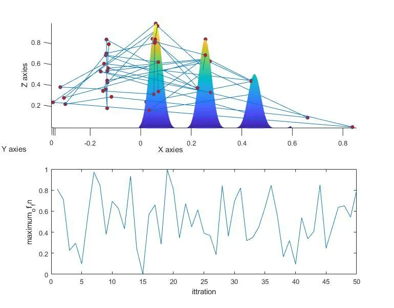values are not confined within the boundries
Statical Behaviour Y-Z View		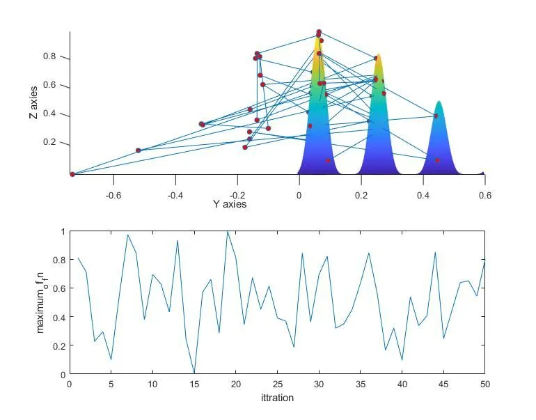due to its varrying nature through the ittraation during optimisation process this results could not truly trusted
Statical Behaviour STUDY TIME		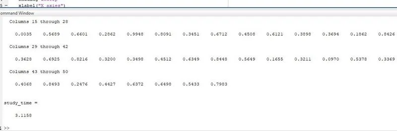STUDY TIME = 3.11sec

• BOUNDED WITHIN RANGE OF DEFINED FUNCTION(0 TO 0.6)

Explanation:

1. Program sarts with clear all close all clc to clear and close the files opened in command window.
2. defining the research space for the stalagmite function using linespace command for x and y values.
3. then the function get_stalagmite is called to calculate the function value over the defined x-y grid.
4. to find the maximum for the function the function is reversed with a negative sign.
5. tic and toc command is used to get the study time taken for the ga to run.
6. for loop is used to run the ga for 50 times using the value in num_case variable defined before the loop .
7. ga is called and stalagmite_fn is optimised for the loop and optimum value with their co-ordinate is stored.
8. ga is defined with function name ,no of variables and boundation for the optimisation is set to 0 to 0.6.
9. for ploting the output results of the stalagmite_function and and optimised values through ga.
10. figure command is used to plot diffrent graphs on same figure window.
11. for the 1st graph using plot command the stalagimte function is ploted and the optimised value is shown.
12. for the 2nd graph plot command is used to plot the optimum value with its corosponding itrration number.
13. xlabel and ylabel is used to define axies names.

PROGRAM

clear all
close all
clc

%defining the research space
x=linspace(0,0.6,150);%150 values in 0 to 0.6 are stored in x
y=linspace(0,0.6,150);%150 values in 0 to 0.6 are stored in y

%num_case is defind to run the ga for the function in loop
num_case=50;%num_case is initialised to 50

%get_stalagmite function is called to callculate the stalagmite function value for the x and y mesh grid values.
F=get_stalegmite(x,y);%F is storing the results from the get_stalagmite function

% TO GET THE MAXIMUM OF THE FUNCTION
%this is done to reverse the stalagmite function results into stalagtite function so that we can find the maximum of the function
f=-F;%f is given the negative values of F

%tic and tac command is used to get the time needed to solve for theresult
tic

%for loop is used to run the genetic alogorithm for several times to get the optomised result
for i=1:num_case % in this case this is made to run 50 times
%genetic algorithm is used to find the minimum of the function
%fopt and its co_ordinates aare returned as results

%Genetic algorithm is bound to serch with in the range of 0 to 0.6 in
%which the plot is made
[inputs,fopt(i)]=ga(@stalagmite_fn,2,[],[],[],[],[0;0],[0.6;0.6])% funtion is passed through ga 
xopt(i)=inputs(1);%1st result of input is the x- co_ordinate of that fopt value.
yopt(i)=inputs(2);%2nd result of input is the y- co_ordinate of that fopt value.
end

%FOR MAXIMUM OF THE FUNCTION
%the optimum varules from the results of ga give minimum value so reverse
%the results with a negative sign
fopt=-fopt%-tive sign is used to find maximum of the function


% timer for the study is stoprd with toc comand
study_time=toc%study_time stored the time value for the ga to solve


%figure window is called with figure comand
figure(1) %for the first figure

%two plots are made in the same figure windom to explain the result
%subplot commnd is used
subplot(2,1,1)%for the 1st subplot
hold on%hold on comand is used to hold the results
surfc(x,y,f)%surface command is used to plot the graph with x values , y values and its corosponding values
shading interp %shape interp is used to get smoth surface with grid lines
xlabel("X axies")% x is labled as x axies
ylabel("Y axies")% y is labled as y axies
zlabel("Z axies")% z is labled as z axies

%now plot command is used to plot the fopt values for the maximum of the function
plot3(xopt,yopt,fopt,'marker','o','markersize',5,'markerfacecolor','r')

%using subplot command to open the second plot for the same figure
subplot(2,1,2)
plot(fopt)%polt comand is used to plot the fopt value 
xlabel("ittration")%% x is labled as ittration
ylabel("maximum_of_fn")% y is labled as maximum_of_fn

RESULTS :

the result from the above condition confined the result within the research space and also there was less variation in the results.

BOUNDED Behaviour TOP View		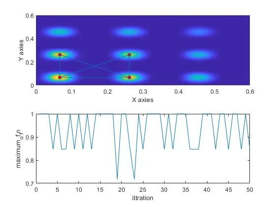the graph show a variation durring the ittration process but the result is not varyin too much
BOUNDED Behaviour X-Z View		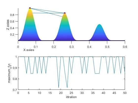values are confined within the boundries defined in the function
BOUNDED Behaviour Y-Z View		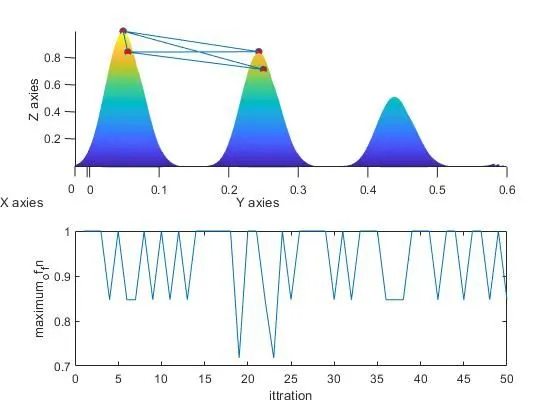due to its less varying nature through the ittraation during optimisation process this results could be likely trusted nad is of some use
BOUNDED Behaviour STUDY TIME		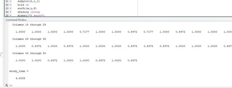STUDY TIME = 4.60sec

• INCREASING POPULATION SIZE

Explanation:

1. Program sarts with clear all close all clc to clear and close the files opened in command window.
2. defining the research space for the stalagmite function using linespace command for x and y values.
3. then the function get_stalagmite is called to calculate the function value over the defined x-y grid.
4. to find the maximum for the function the function is reversed with a negative sign.
5. tic and toc command is used to get the study time taken for the ga to run.
6. for loop is used to run the ga for 50 times using the value in num_case variable defined before the loop .
7. ga is called and stalagmite_fn is optimised for the loop and optimum value with their co-ordinate is stored.
8. options command is used to set the populationsize.
9. ga is defined with function name, no of variables, with boundries of 0 to 0.6 and also populationsize is increased.
10. for ploting the output results of the stalagmite_function and and optimised values through ga.
11. figure command is used to plot diffrent graphs on same figure window.
12. for the 1st graph using plot command the stalagimte function is ploted and the optimised value is shown.
13. for the 2nd graph plot command is used to plot the optimum value with its corosponding itrration number.
14. xlabel and ylabel is used to define axies names.

PROGRAM

clear all
close all
clc

%defining the research space
x=linspace(0,0.6,150);%150 values in 0 to 0.6 are stored in x
y=linspace(0,0.6,150);%150 values in 0 to 0.6 are stored in y

%num_case is defind to run the ga for the function in loop
num_case=50;%num_case is initialised to 50

%get_stalagmite function is called to callculate the stalagmite function value for the x and y mesh grid values.
F=get_stalegmite(x,y);%F is storing the results from the get_stalagmite function

% TO GET THE MAXIMUM OF THE FUNCTION
%this is done to reverse the stalagmite function results into stalagtite function so that we can find the maximum of the function
f=-F;%f is given the negative values of F 

% options are  defined for the ga 
options=optimoptions(@ga); % This returns options with the default values for its fields
options=optimoptions(options,'populationSize',172);% defininng the populationsize 

%tic and tac command is used to get the time needed to solve for theresult
tic

    %for loop is used to run the genetic alogorithm for several times to get the optomised result
for i=1:num_case % in this case this is made to run 50 times
    %genetic algorithm is used to find the minimum of the function
    %fopt and its co_ordinates aare returned as results
    
    %Genetic algorithm is bound to serch with in the range of 0 to 0.6 and
    %definning the populationsize using options of ga functions
    % AND OPTIONS COMMAND IS USED TO INCREASE THE POPULATION SIZE
    %which the plot is made
     [inputs,fopt(i)]=ga(@stalagmite_fn,2,[],[],[],[],[0;0],[0.6;0.6],[],[],options)% funtion is passed through ga 
    xopt(i)=inputs(1);%1st result of input is the x- co_ordinate of that fopt value.
    yopt(i)=inputs(2);%2nd result of input is the y- co_ordinate of that fopt value.
end


%FOR MAXIMUM OF THE FUNCTION
%the optimum varules from the results of ga give minimum value so reverse
%the results with a negative sign
fopt=-fopt%-tive sign is used to find maximum of the function


% timer for the study is stoprd with toc comand
study_time=toc%study_time stored the time value for the ga to solve


%figure window is called with figure comand
figure(1) %for the first figure

%two plots are made in the same figure windom to explain the result
%subplot commnd is used
subplot(2,1,1)%for the 1st subplot
hold on%hold on comand is used to hold the results
surfc(x,y,f)%surface command is used to plot the graph with x values , y values and its corosponding values
shading interp %shape interp is used to get smoth surface with grid lines
xlabel("X axies")% x is labled as x axies
ylabel("Y axies")% y is labled as y axies
zlabel("Z axies")% z is labled as z axies

%now plot command is used to plot the fopt values for the maximum of the function
plot3(xopt,yopt,fopt,'marker','o','markersize',5,'markerfacecolor','r')

%using subplot command to open the second plot for the same figure
subplot(2,1,2)
plot(fopt)%polt comand is used to plot the fopt value 
xlabel("ittration")%% x is labled as ittration
ylabel("maximum_of_fn")% y is labled as maximum_of_fn

RESULT :

the result from these condition of increasing the initial population size with bounded research space give us a more accurate result but the time for optimisating the fuction was too high in comparison to others.

Increasing Population Size TOP View		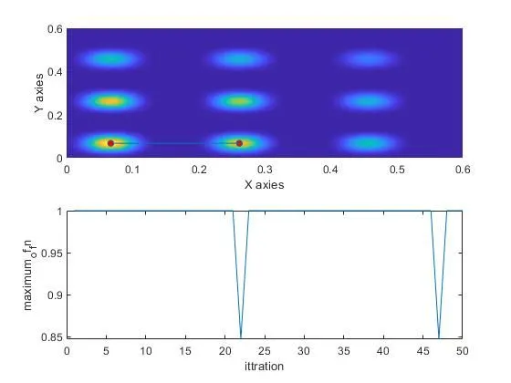the graph show a variation durring the ittration process but the result looks consistance.
Increasing Population Size X-Z View		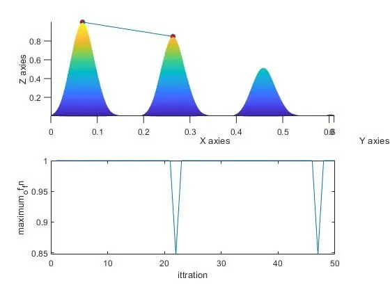values are confined within the boundries defined in the function
Increasing Population Size Z-Y View		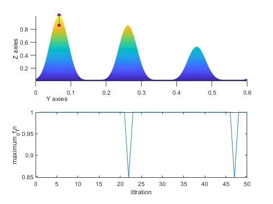due to its nearly consitant nature through the ittraation during optimisation process this results can trusted and it can be seen that its almost accurate
Increasing Population Size Study Time		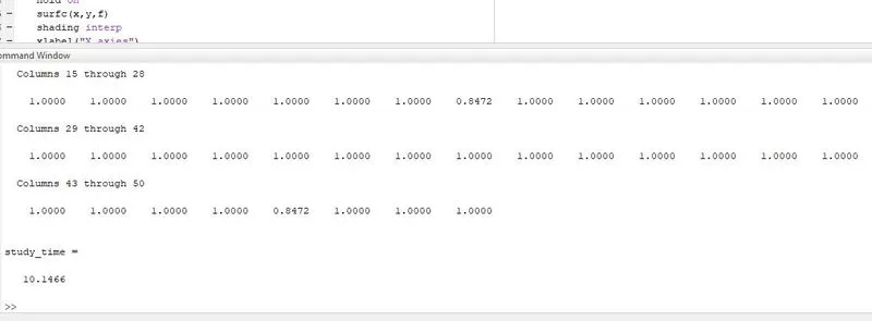STUDY TIME = 10.14sec

FINAL RESULTS :

on comparing the the results from all the 3 conditions applied in the above 3 program the results are listed bellow.

Statical Behaviour	Bounded Behaviour (bounding the function input between 0 to 0.6)	Increasing the Population Size
lowest study time 0f 3.11sec too much variation in the results results are found out of the reseach space.	study time of 4.60sec the variation in the result is less and but accurate	highest study time of 10.14sec there is a consistancy in the results and the results can be seen accurate in the graph.

we can see that the result of the optmisation is improved while changing the condition for the optmisation of the function like

• boundry conditions for the optimisation process
• increasing the population size

But while increasing the condition for optimisation process through ga the time required fro the optimisation also increased a lot.

so we can get the most optimum results form optimisation but the time required for the optimisation is also going to increase with it.

ERROR encountered during running the code.

• the funnction name for calling the get_stalegmite function was missspelled

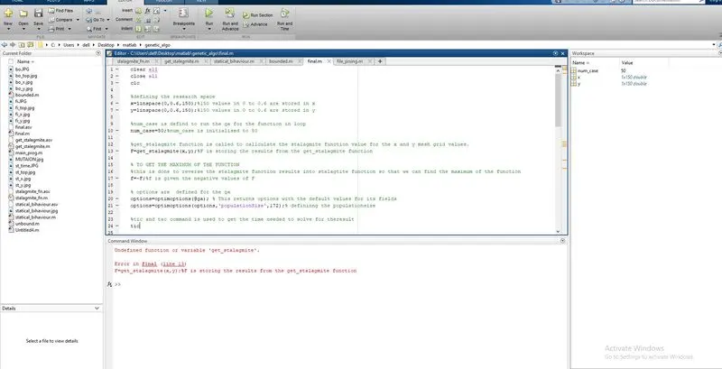
to overcome this the miss spelled name was corrected and the program runed succesfully.