Solving second order ODEs for pendulum motion

AIM: To create the MATLAB program to solve the differential equation for a simple pendulum with damping.

OBJECTIVE: To write a program to simulate and animate the motion of a simple pendulum with damping.

THEORY:

• Differential equations:

A differential equation is an equation which contains one or more terms that are derivatives of one variable (dependent variable) with respect to other variable (independent variable)

`dy/dx = f(x)`

note: 'x' is a independent variable and 'y' is a dependent variable

the derivative represents a rate of change and the differential equation describes a relationship between the quantity that is continuously varying with respect to the change in another quantity.

• Simple pendulum:

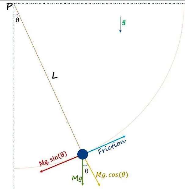
A simple pendulum consists of a mass M hanging from a string of length L from a fixed pivot point P

If the mass of the pendulum is displaced with a initial displacement `theta` then the pendulum will swing back and forth with a periodic motion

angular motion is described by

`tau = Ialpha`

* torque `tau= -mgsintheta . L` , moment of inertia `I=ml^2` and angular acceleration `(d^2 theta)/dt^2`

can be re written as

`-mg sintheta *l=ml^2*(d^2theta)/dt^2`

and this equation can be rearranged as:

`(d^2theta)/dt^2 +g/l sintheta =0`

for `theta` to be small `sintheta ~~ theta`

`(d^2theta)/dt^2 +g/l theta =0`

Damped motion of simple pendulum

In case of damped motion of pendulum, a frictional force opposes the motion of the pendulum which damps the its motion with time

Equation for motion of damped pendulum

• weight of pendulum M can be split in two parts

1. acting away from the center `Mgcostheta` that will be balanced by reaction force acting towards the center.
2. acting in tangential direction of the motion `Mgsintheta`

• frictional force that dampes the motion of pendulum `f= - b.v` (negative sign as it acts against motion,b = damping coeficent , v= velocity)

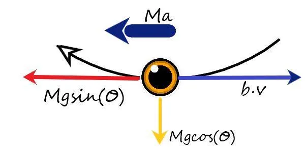
on evaluating the forces in tengential direction

`Ma=-Mgsintheta -b.v`

* as `s = Ltheta` (`(d theta)/dt=1/L (ds)/dt` and `(d^2 theta) /dt^2=1/L (d^2s)/dt`)

so the equation after considering damping becomes

`m(d^2 s)/dt^2 =-b (d s )/dt -Mg.sin theta`

on converting into form of theta

`m (d^2 theta)/dt = -mgsintheta/L-b (d theta)/dt`

`(d^2 theta)/dt +b/M sin theta +g/L sin theta =0`

for `theta` to be small `sintheta ~~ theta`

`(d^2 theta)/dt +b/M sin theta +g/L theta =0`

MATLAB CODE

• MATLAB function to compute differential equation

from the above equation of pendulum

`(d^2 theta)/dt^2 +b/m (d theta )/dt +g/l theta =0`

let `(d theta1)/dt=theta 2` so that `(d^2theta1)/dt^2=(d theta2)/dt`

so we have

1. `(d theta1)/dt=theta 2`

2.`(d theta2)/dt= -b/m(theta2) - g/l(theta1)`

this can be writen as :

`d/dt([[theta1],[theta2]])=[[theta2,],[-b/mtheta2,-g/l theta1]]`

To compute this equation we will use the inbuilt solver ODE45

[t,y] = ode45(fun_name,tspan,y0)

WHERE tspan is time frame (to to tf)

this solves the system of differential equations y′=f(t,y) from t0 to tf with initial conditions y0

ODE_FUNCTION

ode_func is called using the time , initial condition theta_0 and constants of the differential equation

both initial conditions are assigned to theta1 and theta2

using

`d/dt([[theta1],[theta2]])=[[theta2,],[-b/mtheta2,-g/l theta1]]`

to form a matrix equation which is solved using ode45 to get the value of displacement and angular velocity.

%funtion is made to  compute the values of dtheta1(dispacement) and dtheta2(velocity)
%function reqires the values of time,theta,b,g,land m that is passed while calling the function
function [dtheta_dt]=ode_func(t,theta,b,g,l,m) %function "ode_fun" is defined with its input variables and output data(that is velocity and displacement) 
 theta1=theta(1)% theta1 is assingned the 1st value of theta
 theta2=theta(2)% theta2 is assinged the second value of theta
 %as from the solution of matrix 
 dtheta1_dt=theta2;%dtheta1 isequal to theta1
 dtheta2_dt=-(b/m)*theta2 - (g/l)*sin(theta1);%dtheta2 is -(b/m)*theta2 - (g/l)*sin(theta1
 dtheta_dt=[dtheta1_dt;dtheta2_dt];%array of dtheta is assinged the value of matix in two rows
end

IIT GIVE THE VALUE OF DISPLACEMENT AND VELOCITY FOR THE PENDULAM IN FORM OF MATRIX OF TWO ROWS

MAIN PROGRAM TO SIMULATE AND ANIMATE THE PENDULUM MOTION FOR 20 SEC

clear all 
close all
clc

b=0.05;%damping coefficient.
g=9.81;%gravity in m/s2
l=1;%length of the pendulum in m
m=1;%mass of the ball in kg

%initial condition
theta_0=[0;5];%input at t=0(angular displacement(theta);velocity);

%time points
t_span=linspace(0,20,1000);%time span for reviewing the motion (intial value ;final  value; intervals)

%solve ode
%function call to store the time and result of the second order diffrential
%using ode45 function to solve the diffrentiial using values from the ode_func and time that are defined in it
[t,result]=ode45(@(t,theta)ode_func(t,theta,b,g,l,m),t_span, theta_0); %function call TO SOLVE OED USING ode45 and ode_func

%result stores the value of theta1(displacement) and theta2(velocity)for the interval t(time)

ct=1%counter set to 1 (incriment +1 every time for loop) for  geting the  frame recorded
%now we will run the loop to get the value of displacement(theta) for all  intervals of t_span
for j=1:length(result)
        A2=result(j);%variable A2 is assingend the to get the value from result;
        
        
        %as a line has two end points their cordinated are formulated here
        % first coordinate as origin fixed  at (0,0)
        x0=0;%initial co-ordinates
        y0=0;%initial co-ordinates
        
        % second co-ordinate at end of first link as is cosine and sine values
        y1=-l*cosd(A2);%y1 is  length times cos of displacement(theta) (negative for frame  refrence) 
        x1=l*sind(A2);%x1 is  length times sin of displacement(theta)      
        
        %plot is made with two points of line x0 nad  x1
        plot([x0 x1],[y0 y1],'Marker','O','linewidth',2,'MarkerFaceColor','r')
        axis([-0.05 0.05 -1.1 0]) %axies is set for frame x=(-0.05 to 0.05) and y =(-1.1 to 0.05)
        xlabel('x travel  (m)')%labling x axis
        ylabel('y travel  (m)')%labling y axis
        grid on
        pause(0.00003)%time for holding the frame of plot 
        M(ct)=getframe(gcf);%m stores the frame for the animation file 
        ct=ct+1;%counter to get the next frame is increased
    end 



movie(M)% movie function that plays the frames saved in M
videofile = VideoWriter('final.avi','uncompressed AVI');% saving the movie file with name and formate
open(videofile)%open the video file to save the frames in your named file as above
writeVideo(videofile,M)% to write the frame of matrix m in videofile
close(videofile)%close the video file after saving the frames in your named file as above

plot(t,result(:,1))% plot of the displacement with time
hold on
plot(t,result(:,2))%plot of the velocity with time
ylabel("plot value")
xlabel("time")

code explanation

1. Closeall , clear all and clc

to close and clear all the date and plots opened in workspace, clc to clear the command window

2. Assigning the values of the constants

b=0.05 damping coefficient. g=9.81 gravity in m/s2 L=1m length of the pendulum in m M=1mass of the ball in kg

3.Giving initial condition to theta_0 as at t=0 displacement `theta`=0 and angular velocity `omega`=5 rad/sec

4.Setting the time span for which the simulation runs here : for 0 to 20 sec in 1000 intervals ;

5.Calling the ode_func using inbuilt solver ode45 to compute the differential eq.

[t,result]=ode45(@(t,theta)ode_func(t,theta,b,g,l,m),t_span, theta_0);

here ode_func with ode45 solver returns the value of `theta1 and theta2` which in this case is displacement and velocity respectively;

6.counter is set to 1 to get the frames for the animation

7. for loop(runs for the whole length of result)

variable a2 stores each value of result at given interval

to get the co-ordinate of the pendulum pivot is fixed at x=o and y=0 to show gravity downward negative y coordinate is used.

using displacement theta corresponding to the interval second co-ordinate is obtained by `x1=Lsintheta and y1=-Lcostheta`

plot command is used to make the line plot axis is fixed and axis are labeled

pause is used to hold the frame variable m stores the frame using getframe command

counter is increased to save a new frame

loop exit at the end of result

8.Movie file M is then named and saved.

9.plot of displacement and velocity with time is plotted from the result

RESULT

plot of displacement `theta` and angular velocity `omega` with time

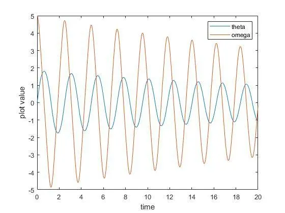
as we can observe that the values of displacement and velocity varies periodically but keeps on decreasing due to the damping in the system.

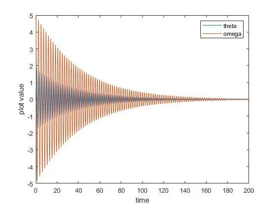
if we increase the time span to 200 sec we can see clearly that the value of displacement and velocity are damped through the motion till it comes to a halt.

ANIMATION FILE : ANIMATION_DAMPED_PENDULUM

ERROR FACED

Animation file cant be saved as the present opned location Directory is not same as the file location

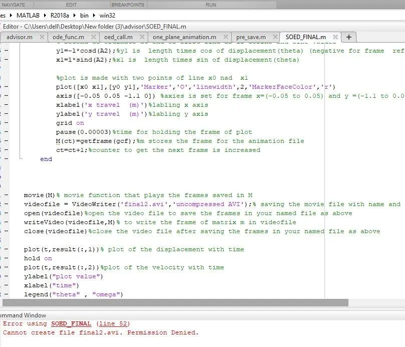
to remove this error current location Directory was changed to the file locaion of the program