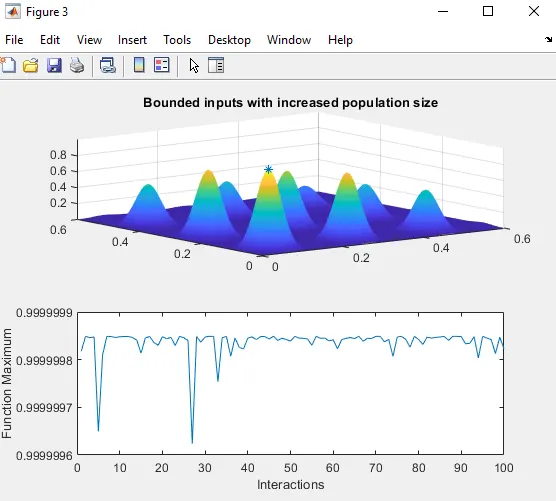
Genetic Algorithm: Optimizing the Stalagmite function to find global maxima of a function.

Objective:

To write a matlab code to optimise the stalagmite function and to find the global maxima of the function.

The objective is to solve for the stalagmite function for given input values and to get the global maxima of the function over the values of input.

Theory:

Before we get on with coding we need to know about optimization, Genetic Algorithm and the stalagmite function which are explained bellow:

Optimization:

fig-1: A system with inputs and outputs

Optimization is an itterative process of making something better/ optimum in a system where there are a set of inputs that undergo a process and given out as a set out outputs, this is a process where we define the subset of inputs for which the system processes the desired/best value of output parameters. The desired/ best values of output are generally the minimum or maximum of the outpu data set or a certain predefined subset of output.

For example an IC engine generates peak torque and power (output parameters) at a specific band of RPM say 2500 to 3000 RPM, then the other inputs and further design will be made to make the most of the engine by keeping the engine running at this RPM band.

The optimization process can be visualized as:

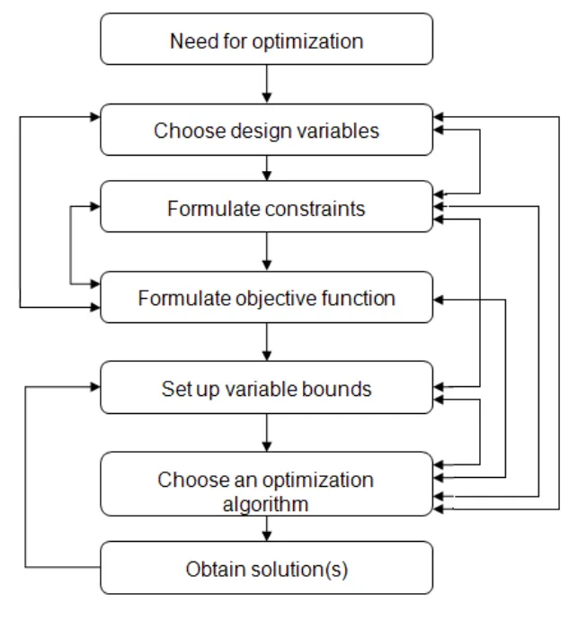
The design variables are the inputs for the system to be designed and the constraints are the limits on the inputs and outputs for the system (such as maximum working temperature for an engine). These inputs are to be fed into the system which is represented by 'Objective Function' this function calculates for the outputs. Depending on the inputs, variable bounds are required to be set up so that the number of itterations are kept in feasible limit. Next a suitable optimization algorithm is selected and run to get solution (Optimal output at set of inputs).

Selection of optimization algorithm is problem specific as each problem has different contstraints and different objective functions. And no single algorithm is suitable for all such conditions.

Some of the optimization algoritms are:

1. Single Variable opt. algorithm (Direct Method, Gradient based method)

2. Multi-variable opt. algorithm

3. Constrained opt. algorithm (inputs search is nlimited to a defined region)

4. Specialized opt. algorithms (integer programming, geometric programming)

5. Non-traditional opt. algorithms:(Genetic algorithm, Simulated annealing)

Genetic Algorith:

Genetica Algorithm is a search based optimization algorith that uses probabilistic approach based on natural selectiopn theory. The GA is generally used tio find the minima of a given function.

The flow chart of GA processes:

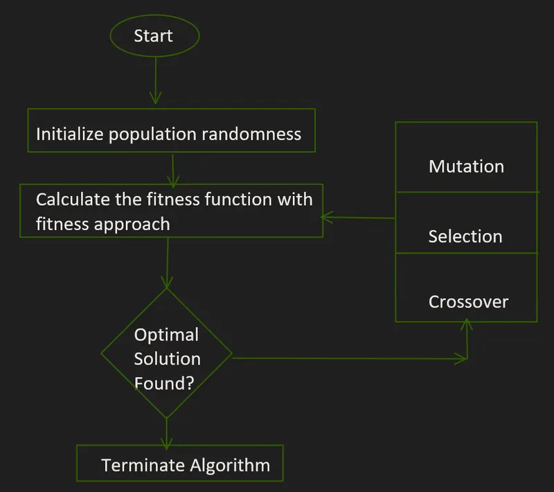
The algorithm is initated by providing a random or a predifind set to select the random inputs for the fitness function. Then, we have a pool of solutions represented by population and each individual has a fitness value assigned based on the objective function. Now these individuals undergo Selection, Mutation, and Reproductive Crossover as in natural genetics and reproduction. Also as in natural selection, Individual with greater fittness value have greater chance of reproduction and passing on the genes in next generations. This process is then repeated over a various generations till there are negligible changes in the outputs i. e. when we reach convergence. The termination of this loop is defined by how close to exact value of optimal output is required.

In Selection Parents are selected from sample data points, favouring greater fitness value individuals. The selection is a random process and is simulated using 'Roulette Wheel' selection method.

A Roulette wheel is like a pie chart with a fixed point to pick the individuals, where the individuals with greaer fittness are assigned grater angle hence a greater fittness value individuals represent a proportionate greater slice of the pie. This wheel is then spinned against a fixed point

Cross-over is a process of two parents solutions and producing the child from them.

Mutation is carried out to mainteain genetic diversity from one generation population of chromosomes to next one. If this is not done, the chromosomes become too similar to each other and the convergence takes place soon.

syntax ga in Matlab:

1. [inputs, fval] = ga(@stalagmite, 2)

Above command will calculate for the genetic algorithm mof the function- 'stalagmite' with '2' input variables, population size remains to be 50 here.

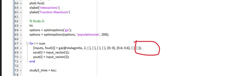
2. [inputs, fout(i)] = ga(@stalagmite, 2, [ ], [ ], [ ], [ ], [0; 0], [0.6; 0.6], [ ], [ ]);

This command will calculate for GA of 'stalagmite' for inputs ranging from 0 to 0.6 in both x and y directions, this is done by defining the lower and upper bounds by [0; 0], [0.6; 0.6], also with default population of 50.

3. The population size is defined by using 'options' in the GA line.

options = optimoptions('ga');
options = optimoptions(options, 'populationsize', 200);

[inputs, fout(i)] = ga(@stalagmite, 2, [ ], [ ], [ ], [ ], [0; 0], [0.6; 0.6], [ ], [ ], options);

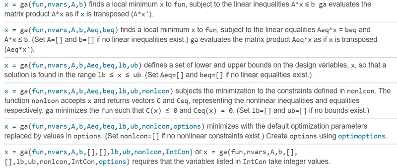
pic source: matlab help doc 'ga'

Stalagmite function:

Fig: Stalactite and stalagmite in a cave.

As shown in above fig, a stalagmite refers to the upward growing pile of miniral diposit in a cave due to the seapage of water over a long period of time.

Mathematically, a stalagmite function generates values over a surface that resembles cave stalagmits and is used to find the local and global maxima.

Here, in this programme, we are evaluating a stalagmite function using GA-Genetic Algorith (an inbuit optimization method).

Our objective here is to create a surface plot where, the inputs are in x and y direction and the function output is in z direction.

Such as: `z = f(x,y)`

But, the GA gives out the minima of a function. So in order to find the stalagmite function maxima we define another function`z = F=-f(x,y)` and then GA on this function. This will calculate for the minima of the negative value of our required function and hence give out the required maxima`

The Stalagmite function: `f(x, y) = f_(1x) f_(1y) f_(2x) f_(2y)`

`f_(1x) = (sin(5.1pix + 0.5))^6`

`f_(1y) = (sin(5.1piy + 0.5))^6`

`f_(2x) = exp[-4ln(2) (x-0.0667)^2/0.64]`

`f_(2y) = exp[-4ln(2) (y-0.0667)^2/0.64]`

Referances:

1. https://skill-lync.com/knowledgebase/genetic-algorithm-explained

2. https://www.tutorialspoint.com/genetic_algorithms/genetic_algorithms_fundamentals.htm

Code:

Main code:

clear all
close all
clc
% Defining search space
x = linspace(0, 0.6, 150);
y = linspace(0, 0.6, 150);
% Creating 2D mesh
[xx yy] = meshgrid(x, y);
% Evaluating the stalagmite function
for i = 1: length(xx)
    for j = 1:length(yy)
        input_vector(1) = xx(i, j);
        input_vector(2) = yy(i, j);
        f(i, j) = stalagmite(input_vector);
    end
end
num = 100;
% Study-1
tic                                               % Starts Recording time 
for i = 1:num
    [input_vector, fout(i)] = ga(@stalagmite, 2);
    xout(i) = input_vector(1);
    yout(i) = input_vector(2);
end
study1_time = toc;                                % Ends recording time are saves for the recorded value in Study1_time 
% Plotting FOR Study-1
figure(1)
subplot(2, 1, 1)                                  % Plots 2 different subplots in one window Selecting for 1st subplot here
surfc(xx, yy, -f)                                 % Surface ploting
hold on                                           % To overlap 2 plots
shading interp                                    % Removes lines from the graph
plot3(xout, yout, -fout)                          % 3D Plot
title('Unbounded inputs') 
subplot(2, 1, 2)                                  % Selecting for 2nd subplot
plot(-fout)                                       % Ploting for Foptimized against interactions
xlabel('interactions')
ylabel('Function Maximum')
hold off                                          % Terminating hold to clear plot window for next study
[inputs, fval] = ga(@stalagmite, 2);

% Study-2: with upper bound and lower bound
tic                                               % Starts Recording time
for i = 1: num
    [inputs, fout(i)] = ga(@stalagmite, 2, [], [], [], [], [0; 0], [0.6; 0.6], [ ], [ ]);         % Defining lower and upper bounds for the ga search space.
    xout(i) = inputs(1);
    yout(i) = inputs(2);
end
study2_time = toc                                 % Ends recording time are saves for the recorded value in Study2_time
% Plotting FOR Study-2
figure(2)
subplot(2, 1, 1)
surfc(x, y, -f)
shading interp
hold on
plot3(xout, yout, -fout, 'marker', '*')
title('Bounded Inputs')
subplot(2,1,2)
plot(-fout)
xlabel('Interactions')
ylabel('Function Maximum')
hold off

% Study-3: 
tic
options = optimoptions('ga');                                               % Assiugning value to options to be fed in GA command.
options = optimoptions(options, 'PopulationSize', 300);      % Specifying for the population size.
for i = 1:num
    [inputs, fout(i)] = ga(@stalagmite, 2, [], [], [], [], [0; 0], [0.6; 0.6], [], options);        % Defining lowew and upper bound for search space and increasing population size to 300
    xout(i) = inputs(1);
    yout(i) = inputs(2);
end
study3_time = toc
% Plotting FOR Study-3
figure(3)
subplot(2,1,1)
surfc(x, y, -f)
shading interp
hold on
plot3(xout, yout, -fout, 'marker', '*')
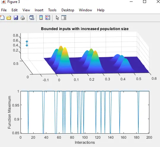
title('Bounded inputs with increased population size')
subplot(2,1,2)
plot(-fout)
xlabel('Interactions')
ylabel('Function Maximum')
hold off

Function Code:

function code for stalagmite function:

function Z = stalagmite(input_vector)
x = input_vector(1);                            % Defining values for x and y to be used in function calculation.
y = input_vector(2);
f1x = (sin((5.1*pi*x) + 0.5))^6;
f1y = (sin((5.1*pi*y) + 0.5))^6;
f2x = exp(((-4)*log(2)*(x- 0.0667)^2)/0.64);
f2y = exp(((-4)*log(2)*(y- 0.0667)^2)/0.64);
Z = -(f1x* f1y* f2x* f2y);                      % Assigned '-'ve value for the function as our objective is to find the maxima
end

Code Comments:

1. The search space is defined by asigning values to 'x' and 'y' with 'linspace' command creating arrays for 'x' and 'y'
2. [xx yy] matrix is defined using 'meshgrid(x, y)' to generate values for the surface plot.
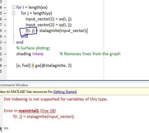
3. 2 for loops are used to calculate for the stalagmite function for each value in [xx yy], for i= 1:length(xx) selects value of 'x' and the subordinate for j = 1:length(yy) picks up the values of y and here the function stalagmite is calculated for selected values of 'x and 'y' hence by the end of both the for loops, all values of stalagmite are calculated and stored as 'f'

Study1:

1. No. of instances are defined by 'num = 100'
2. 'tic' and 'toc' is used to record for the time for study1
3. The for loop is used to solve for the genetic algorithm by for i= 1:num
4. [inputs, fval] = ga(@stalagmite, 2) runs genetic algorithm for all given instances and xout and yout arrays are defined for the ploting of optimized 'x', 'y', 'fout' in 3D plot.
5. 'subplot(2, 1, 1)' is used to plot two different plots in one figure(1) window followed by a surfc(xx, yy, -f) that plots a surface plot and plot3(xout, yout, -fout) ploting a 3D plot. Here hold on is used to overlap these two plots. Here, to get a positive plot, '-f' is used in surface plot because the function stalagmite is defined -ve.
6. subplot(2, 1, 2) is used to select for the 2nd plot in the figur(1) window and plot(-fout) is use to plot for the optimized f against interactions.

Study2:

1. tic and toc is used to record time for study 2
2. Here, [inputs, fout(i)] = ga(@stalagmite, 2, [ ], [ ], [ ], [ ], [0; 0], [0.6; 0.6], [ ], [ ]); calculates for GA with inputs bounded to 0 to 0.6 in both x and y.
3. same sequence of plotting commands is used for figure(2) as in figure(1)

Study3:

1. tic and toc records for study 3 time.
2. 'options' is defined for the GA to set the population size to 300 with following sequence:

• options = optimoptions('ga');
  options = optimoptions(options, 'populationsize', 300);
• for i = 1:num
• [inputs, fout(i)] = ga(@stalagmite, 2, [ ], [ ], [ ], [ ], [0; 0], [0.6; 0.6], [ ], [ ], options);

Function stalagmite:

• x and y variables are defined by input_vector()
• the formulae are used for getting the four base functions.
• The main function is calculated using these four functions and is assigned with '-'ve sign as we are computing for the maxima and the GA calculates for minima.

Errors:

1. wrote '.' in place of ','

Results:

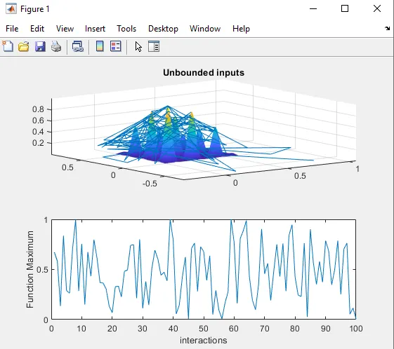
Study1:

Time Lapsed = 7.4311 sec

Much broader variation of function maxima

Study2:

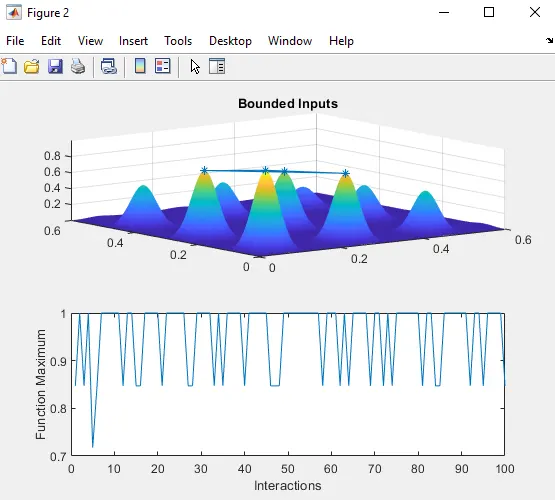
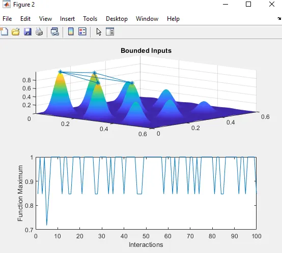
Time lapsed = 10.4682 sec

As it can be seen in figure(2) plots, the function maximum is in a shorter band than study1

Study3:

Time Lapsed = 43.762 sec

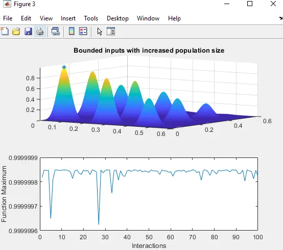
In this case the function maximum is in a very very short bandwidth as shown in figure(3) plots, variation is in `10^(-7)`place hence giving out a very very close resemblence to absolute function maximum