Rankine cycle Simulator
Objective: To wite a matlab code to simulate the Rankine Cycle.
The power plats describes the processes followed in most of thermal power plants that use steam operated heat engines. Here, in this project we are tracing for the thermodynamic state variables to map the rankine cycle for given input conditions.
Theory:
Rankine cycle and its usage:
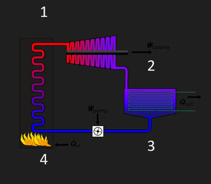
Rankine cycle is used to predict the performance of a steam turbine cycle where the heat is added to the working fluid (Water/ Steam) at const. pressure which expands in turbine giving out heat and doing work on the shaft. This is a closed loop cycle and the fluid here is recirculated through a condensor. As the fluid has to overcome pressure loses to flow through the cycle, a feader pump is used to increase the presure prior heating the water.
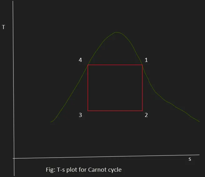
Rankine cycle closely resemble the carnot vapor cycle but due to practical limitation of the pump which can only handle water and the steam turbine that is most economical to run with superheated steam, causes slight deviation from the ideal cycle.
T-s and h-s plots for a Carnot Cycle amd Rankine Cycle:
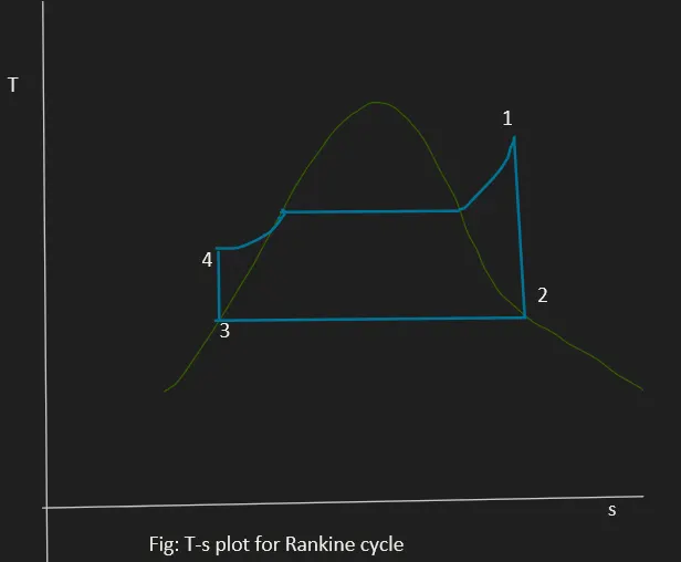
Rankine Cycle processes:
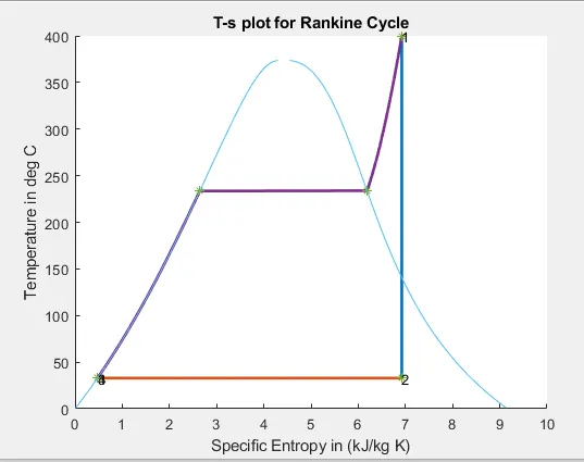
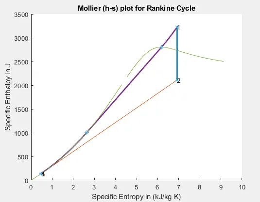
- 1-2 is isentropic expansion, work is done by the steam on the shaft while it expands througth the turbine.
- 2-3 is constant temp. heatr rejection process. This is done to condence the saturated steam from turbine exit to water.
- 3-4 is isentropic work addition, here the pump acts on water, increasing its pressure.
- 4-1 is a isobaric heat addition processes, in this processes, the water is converted in to saturated steam as it crocesses the critical point line and the heat is added to the steam till it is superheated increasing the temp. and enthalpy of the steam.
XSteam: XSteam file is a matlab file that resembles the steam tables and like steam tables, has the properties of water such as entropy, enthalpy for liquid and solid state for a given pressure and temperature range.
Formulae:
Workdone by Turbine:
`W_t = h_(i) - h_o`
Workdone by the pump:
`W_p = v_p(p_o - p_i)`
Net Workdone:
`W_(nt) = W_t - W_p`
Heat Input:
`Q_(i) = h_(oboilr) - h_(iboilr)`
Thermal Efficiency:
`eta = W_(nt)/Q_i`
Back work ratio:
`b.w.r. = W_p/W_t`
Referances:
- https://en.wikipedia.org/wiki/Rankine_cycle#:~:text=The%20Rankine%20cycle%20is%20a,work%20while%20undergoing%20phase%20change.
- https://drive.google.com/file/d/1RK_fvrOj38CIaQvmLT1S3daqHnxKCGU-/vie
Code:
% Rankine cycle simulator
clear all
close all
clc
% Given Inputs:
T1 = input('Enter the Turbine inlet temp in deg C');
p1 = input('Enter the Turbine inlet pressure in bar');
p2 = input('Enter the Turbine outlet pressure in bar');
% state variable are: T (Temperature), p (pressure), h (Enthalpy), s (entropy)
% 1-2 isentropic expansion in turbine:
s1 = XSteam('s_pT', p1,  T1);
s2 = s1;                                                        % Isentropic process
h1 = XSteam('h_pT', p1, T1);
T2 = XSteam('T_ps', p2, s2);
x2 = XSteam('x_ps', p2, s2);
h2 = XSteam('h_px', p2, x2);
% 2-3 is const pressure heat rejection
p3 = p2;
T3 = T2;
s3 = XSteam('sL_p', p3);
h3 = XSteam('hL_T', T3);
%for the 2-3 curve calculation:
sspace = linspace(s3, s2, 1000);
for k = 1:length(sspace)
    hspace(k) = XSteam('h_ps', p2, sspace(k));
end
 % 3-4 isentropic compression:
p4 = p1;                                                % pumping water to be fed in turbine: p1 = p4
s4 = s3;
Cp = XSteam('Cp_ps', p4, s4);
Cv = XSteam('Cv_ps', p4, s4);
gamma = Cp/Cv;
Vp = XSteam('vL_p', p4);
Wp = Vp* (p4-p3);
h4 = h3+ Wp;
T4 = T3+ ((h4-h3)/Cv);
% 4-1 is isobaric heat addition
TL4 = XSteam('Tsat_p', p4);
sL4 = XSteam('sL_p', p4);
hL4 = XSteam('hL_p', p4);
TV4 = XSteam('Tsat_p', p4);
hV4 = XSteam('hV_p', p4);
sV4 = XSteam('sV_p', p4);
%for the 4-1 curve calculation:
Tboiler = linspace(T4, T1, 1000);
for j = 1:length(Tboiler)
    scurve(j) = XSteam('s_pT', p4, Tboiler(j));
    hcurve(j) = XSteam('h_pT', p4, Tboiler(j));
end
% For the saturated line:
temp_range = linspace(1, 500, 1000);
for i = 1: length(temp_range)
    hLsat(i) = XSteam('hL_T', temp_range(i));
    sLsat(i) = XSteam('sL_T', temp_range(i));
    hVsat(i) = XSteam('hV_T', temp_range(i));
    sVsat(i) = XSteam('sV_T', temp_range(i));
end
% Displaying the state variables at different stages
fprintf('At state1- Turbine Inlet');
fprintf('n p1 is: %f bar', p1);
fprintf('n T1 is: %f C', T1);
fprintf('n h1 is: %f', h1);
fprintf('n s1 is: %f', s1);
fprintf('n At state 2 - Turbine Outlet, Condensor inlet');
fprintf('n p2 is: %f bar', p2);
fprintf('n T2 is: %f C', T2);
fprintf('n h2 is: %f', h2);
fprintf('n s2 is: %f', s2);
fprintf('n At state 3 - Condensor Outlet, Pump Inlet');
fprintf('n p3 is: %f bar', p3);
fprintf('n T3 is: %f C', T3);
fprintf('n h3 is: %f', h3);
fprintf('n s3 is: %f', s3);
fprintf('n At state 4- Pump Outlet Boiler Inlet');
fprintf('n p4 is: %f bar', p4);
fprintf('n T4 is: %f C', T4);
fprintf('n h4 is: %f', h4);
fprintf('n s4 is: %f', s4);
% Workdone
Wt = h1 - h2;
Wnet = Wt - Wp;
bwr = Wp/Wt;
fprintf(' n Back Work Ratio is: %f', bwr);
fprintf('n Net Work Output is: %f', Wnet); disp('J')
% Heat supplied
Qin = h1- h4;
% Thermal Efficiency:
n = (Wnet/ Qin)* 100;
fprintf('n Thermal Efficiency is: %f', n); disp('%');
% plotting
figure(1)
hold on
plot([s1 s2], [T1 T2], 'linewidth', 2)
plot([s2 s3], [T2 T3], 'linewidth', 2)
plot([s3 s4], [T3 T4], 'linewidth', 2)
% 4-L curve
plot(scurve, Tboiler, 'linewidth', 2)
% V-1 curve
plot([s1 s2  s3 s4 sL4 sV4], [T1 T2 T3 T4 TL4 TV4], '*')
plot([sLsat, sVsat], [temp_range, temp_range])
text(s1, T1, '1')
text(s2, T2, '2')
text(s3, T3, '3')
text(s4, T4, '4')
xlabel('Specific Entropy in (kJ/kg K)')
ylabel('Temperature in deg C')
title('T-s plot for Rankine Cycle')

figure(2)
hold on
plot([s1 s2], [h1 h2], 'linewidth', 2)
%2-3 curve
plot(sspace, hspace)
plot([s3 s4], [h3 h4], 'linewidth', 2)
% 4-1 curve
plot(scurve, hcurve, 'linewidth', 2)
plot([sLsat, sVsat], [hLsat, hVsat])
plot([s1 s2 s3 s4 sL4 sV4], [h1 h2 h3 h4 hL4 hV4], '*')
text(s1, h1, '1')
text(s2, h2, '2')
text(s3, h3, '3')
text(s4, h4, '4')
xlabel('Specific Entropy in (kJ/kg K)')
ylabel('Specific Enthalpy in J')
title('Mollier (h-s) plot for Rankine Cycle')
Code Comments:
- The given inputs are defined through 'input' command.
- To calculate for the state variables the data from XSteam file is extracted with 'XSteam('hL_p', p1);' - XSteamlooks for hL_p variable for the referance value of 'p1' in this case. Each variable is defined for its function name to be called for in the XSteam file.
- Now the state variables Temperature(T), pressure(p), Enthalpy( h) and Entropy(s) are calculated based on the thermodynamic processes of the cycle.
- To calculate for the intermediate state variables between the stage points, for loops are used such as:
'sspace = linspace(s3, s2, 1000);
for k = 1:length(sspace)
hspace(k) = XSteam('h_ps', p2, sspace(k));
end'
here, the base referance state variable is defined first with a linspace command and then a for loop is used to extract the data from XSteam for each instance of referance variable.
- similarly the process 4-1 is traces with a for loop extracting data points for entropy and enthalpy with boiler inlet pressure and boiler temp range as referance inputs.
- To trace for the saturation curve on the plots, a for loop is used to extract the Saturation Entropyand Enthalpy w.r.t. Temperature.
- The net workdone, turbinne work, pump work, heat supplied, Thermal Efficiency and the back work ratio are calculated using the above mentioned formulae.
- 2 plots are generated figure() command to make different plot windows.
- hold on is used to overlap a sequence of plot commands in a single window.
Errors:
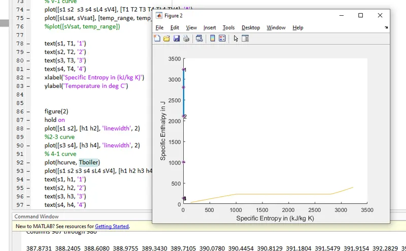
1. Improper use of variables in plot command:
Results:
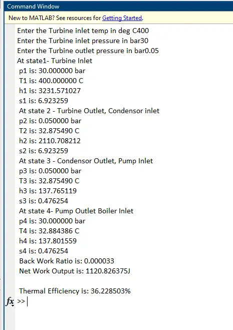
Enter the Turbine inlet temp in deg C400
Enter the Turbine inlet pressure in bar30
Enter the Turbine outlet pressure in bar0.05
 At state1- Turbine Inlet
 p1 is: 30.000000 bar
 T1 is: 400.000000 C
 h1 is: 3231.571027
 s1 is: 6.923259
 At state 2 - Turbine Outlet, Condensor inlet
 p2 is: 0.050000 bar
 T2 is: 32.875490 C
 h2 is: 2110.708212
 s2 is: 6.923259
 At state 3 - Condensor Outlet, Pump Inlet
 p3 is: 0.050000 bar
 T3 is: 32.875490 C
 h3 is: 137.765119
 s3 is: 0.476254
 At state 4- Pump Outlet Boiler Inlet
 p4 is: 30.000000 bar
 T4 is: 32.884386 C
 h4 is: 137.801559
 s4 is: 0.476254
 Back Work Ratio is: 0.000033
 Net Work Output is: 1120.826375J

 Thermal Efficiency is: 36.228503%
>>
T-s Plot:
h-s Plot:
Command Window: