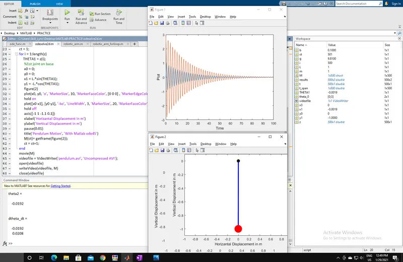
Solving second order ODEs

Problem Statement:

To write a code that solves 2nd order ODE for simulating the pendulum motion and to create the animation of the pendumum.

Theory:

The ODEs (Ordernary Differential Equatioins) are very common in solving engineering problems and these can be solved using Matlab command 'ode45'.

In this case we are soloving the ODE that calculates for the change in pendulum angle w.r.t. time and the rate of change of the angle by solving for a 2nd order ODE.

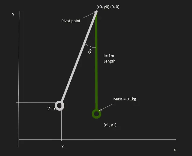
Here,

`theta` : the deflection angle

L: Length of pendulum (1m)

m: Mass of pendulum (1kg)

g = acc. due to gravity (9.81`m/s^2`)

b = damping coefficient (0.1)

Initial agitation velocity: 5m/s

When the pendulum is agitated it moves by an angle `theta` but due to gravity decelerates as it moves outwards and returns towards center and thus oscillates.

If there was no resistance for this motion it would continue indefinatly but the surrounding air, bearing friction provides resistance to this motion hence damps the motion.

The damping is calculated using the damping coefficient(b).

`(d(theta))/ dt` : change in`theta`w.r.t. time

`(d^2(theta))/(d^2t)` : rate of change `theta` w.r.t. time

Equation of motion for the pendulum:

`(d^2(theta))/(d^2t)+b/m(d(theta))/(dt) + g/L sin(theta)`

this equation defines the values of `theta`w.r.t. tim

ode45 command:

[t,x] = ode45(@(t,x) 2*t(A), [0, 5](B), y0(C))
In this line ode45 is solving for equation denoted by(A), in the interval of(B): 0 - 5, for the initial condition of (C): y0
ode45 solves for 1st order ODEs. This is very useful to get values of variables defined by ODEs with respect to time, r.p.m, velocity etc in a matrix form.

Code:

% To write a code to solve 2nd order ODE
clear all
close all
clc
% Input Parameters:
g = 9.81;                                %Gravity in 'm/s^2'
b = 0.1;                                 % Damping co-efficient
L = 1;                                   % Length of the pendulum in 'm'
m = 1;                                   % mass of pendulum
% Initial condition:
theta_0 = [0; 3];                        % Initial [Displacement; Velocity] (a calumn matrix)
t_span = linspace(0, 100, 500);          % Time instances
% Solving for ODE
[t, results] = ode45(@(t, theta) ode_func(t,theta,b,g,L,m), t_span, theta_0);

figure(1)
plot(t, results(:, 1))
hold on
plot(t, results(:, 2))
xlabel('Time')
ylabel('Plot')
z = results(:,1);
ct = 1;
for i = 1:length(z)
    THETA1 = z(i);
     %1st joint on base 
     x0 = 0;
     y0 = 0;
     x1 = L.*sin(THETA1);
     y1 = -L.*cos(THETA1);
     figure(2)
     plot(x0, y0, 'o', 'MarkerSize', 10, 'MarkerFaceColor', [0 0 0] , 'MarkerEdgeColor', [1 1 0])
     hold on 
     plot([x0 x1], [y0 y1], '-bo', 'LineWidth', 3, 'MarkerSize', 20, 'MarkerFaceColor', 'r', 'MarkerEdgeColor', 'r', 'MarkerIndices', 2)
     hold off
     axis([-1 1 -1.1 0.1])
     xlabel('Horizantal Displacement in m')
     ylabel('Vertical Displacement in m')
     pause(0.01)
     title('Pendulum Motion', 'With Matlab ode45')
     M(ct)= getframe(figure(2));
     ct = ct+1;
end
movie(M)
videofile = VideoWriter('pendulum.avi', 'Uncompressed AVI');
open(videofile)
writeVideo(videofile, M)
close(videofile)

Code Comments:

1. The Input parameters are defined in the code as mentioned above.

2. The function programme is called upon to calculate for the theta variation and plots are generated for the displacement and velocity of the pendulum.

3. A for loop is used to calculate the co=ordinates of the pensulum bob at each instance of `theta`and an array 'z' is defined for the displacement values from the result matrix and this array is used for the co-ordinates calculation.

4. negative sign is used for y- coordinate to show the hing at top and bob at bottom.

5. the plot command is used twice to show the line and different markes at the end points with a hold on and hold off command to show both the plots at once for an instance and then to clear the plot window for next instance.

6. the plot is completed by providing annotation thourh xlabel, title commands.

7. To compile the movie, a counter (ct) is used to record the plot for a single instance of `theta`and then with M(ct) = getframe(figure(2)) is used to combnine all the plot frames.

on completion of the for loop, The commands movie(M), videoWriter, open , write and close are used to record the movie and save the vedio file for given name.

Function Code:

function [dtheta_dt] = ode_func(t, theta, b, g, L, m)

theta1 = theta(1)                   %Defining 2nd order ODE in 2 seperate 1st order ODES
theta2 = theta(2)
dtheta1_dt = theta2;
dtheta2_dt = -(b/m)*theta2 - (g/L)*sin(theta1);  % Motion Equation
dtheta_dt = [dtheta1_dt; dtheta2_dt]             % Resulting matrix
end

Here, as the ode45 command solves only for 1st order ODE, we have defined the function with two 1st order ODEs that represent the main 2nd order ODE motion equation.

Errors in Programme:

1. hold on and hold off improper use:

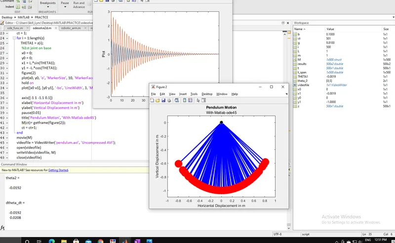
2. Wrong usage of Markers, MarkerIndices and placement in plot command

3. Not incerting counter(ct) at the begining of for loop : video not recorded

Results:

Vedio Link: https://youtu.be/p306LDVioZ4