Week 4 - Genetic Algorithm

Genetic algorithm:

Genetic algorithms are an approach to optimization and learning based loosely on principles of biological evolution, these are simple to construct, and its implementation does not require a large amount of storage, making them a sufficient choice for an optimization problems. Optimal scheduling is a nonlinear problem that cannot be solved easily yet, a GA could serve to find a decent solution in a limited amount of time. Genetic algorithms are inspired by the Darwin’s theory about the evolution “survival of fittest”, it search the solution space of a function through the use of simulated evolution (survival of the fittest) strategy.

Genetic algorithms have been shown to solve linear and nonlinear problems by exploring all regions of the state space and exponentially exploiting promising areas through the application of mutation, crossover and selection operations to individuals in the population.

Syntax for ga in MATLAB:

x = ga(fun,nvars,A,b,Aeq,Beq, lb, ub, nonlcon, IntCon, options)

where,ga finds a local unconstrained minimum, x,

to the objective function, fun,subject to the linear equalities Aeq*x = beq and linear inequalities A*x ≤ b.

nvars is the dimension (number of design variables) of fun.

lb and ub are a set of lower and upper bounds on the design variables, x, so that a solution is found in the range lb ≤ x ≤ ub.

The function nonlcon accepts x and returns vectors C and Ceq, representing the nonlinear inequalities and equalities respectively.

x minimizes with the default optimization parameters replaced by values in options.The default population taken is 50.

variables listed in IntCon take integer values.

A code in MATLAB to optimise the stalagmite function and find the global maxima of the function:

Note that the genetic algorithm is designed to return the global minima values and there is a modification to get the maximas as solution.

%%Stalagmite fitness function as defined by the equations given.

function [f] = stalagmite(input_vector)
x = input_vector(1);
y = input_vector(2);

f1_x = [sin(5.1*pi*x+0.5)]^6;
f1_y = [sin(5.1*pi*y+0.5)]^6;
f2_x = exp(-4*log(2)*(((x-0.0667)^2)/0.64));
f2_y = exp(-4*log(2)*(((y-0.0667)^2)/0.64));
%% To get the maxima a negative sign is introduced and to correct the sign an additional %% -ve sign is used in the main code.
[f] = -(f1_x.*f2_x.*f1_y.*f2_y);
end

Main program for finding maxima for the function:

clear all 
close all
clc

%defining the search space
x = linspace(0,0.6,150);
y = linspace(0,0.6,150);

%creating a 2D mesh:
[xx yy] = meshgrid(x,y);

%Evaluating the stalagmite function:
for i = 1:length(xx)
    for j = 1:length(yy)
        input_vector(1) = xx(i,j);
        input_vector(2) = yy(i,j);
    f(i,j) = stalagmite(input_vector);
    end
end

%case1 - statistical behaviour:
tic
%defining the number of iterations to be carried out.
num_cases = 50;
for i = 1:num_cases;
     [inputs,fopt(i)] = ga(@stalagmite,2);
     xopt(i) = inputs(1);
     yopt(i) = inputs(2);
end
study1time = toc
%% -ve sign is used to correct the value of maximas obtained from the stalagmite %%function
F = -f;

%% Plotting the curve along the data points acquired and plotting the maximas in each iteration to see the changes in the maxima values.
figure(1)
subplot(2,1,1)
hold on
surfc(x,y,F);
shading interp;
plot3(xopt,yopt,-fopt,'marker','o','markersize',5,'markerfacecolor','r');
title('unbounded inputs')
xlabel('x')
ylabel('y')
zlabel('f')
subplot(2,1,2)
plot(-fopt)
xlabel('Iterations')
ylabel('Function maximum')

output:

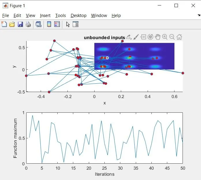
Here as we can observe there are a lot of local maxima and it is difficult to get an optimized value for the global maxima.

The value of minima or maxima can be optimized further by introducing lower and upper bounds and increasing the population that the genetic algorithm evaluates.

The code for the optimization using these techniques is given below:

clear all 
close all
clc

%defining the search space
x = linspace(0,0.6,150);
y = linspace(0,0.6,150);

%creating a 2D mesh:
[xx yy] = meshgrid(x,y);

%Evaluating the stalagmite function:
for i = 1:length(xx)
    for j = 1:length(yy)
        input_vector(1) = xx(i,j);
        input_vector(2) = yy(i,j);
    f(i,j) = stalagmite(input_vector);
    end
end

%case1 - statistical behaviour:
tic
num_cases = 50;
for i = 1:num_cases;
     [inputs,fopt(i)] = ga(@stalagmite,2);
     xopt(i) = inputs(1);
     yopt(i) = inputs(2);
end
study1time = toc
F = -f;
% plotting
figure(1)
subplot(2,1,1)
hold on
surfc(x,y,F);
shading interp;
plot3(xopt,yopt,-fopt,'marker','o','markersize',5,'markerfacecolor','r');
title('unbounded inputs')
xlabel('x')
ylabel('y')
zlabel('f')
subplot(2,1,2)
plot(-fopt)
xlabel('Iterations')
ylabel('Function maximum')


%Study2 = bounded iterations with upper and lower bound
options = optimoptions('ga','populationsize',50)
tic
num_cases = 50;
for i = 1:num_cases;
    [inputs,fopt(i)] = ga(@stalagmite,2,[],[],[],[],[0 0],[0.6 0.6]);
    xopt(i) = inputs(1);
    yopt(i) = inputs(2);
end
study2time = toc

%plotting
figure(2)
F = -f;
subplot(2,1,1)
hold on
surfc(x,y,F)
plot3(xopt,yopt,-fopt,'marker','o','markersize',5,'markerfacecolor','r');
title('Bounded inputs')
xlabel('x')
ylabel('y')
zlabel('f')
subplot(2,1,2)
plot(-fopt)
xlabel('Iterations')
ylabel('Function maximum')

%study3 = Bounded values with modified population size:
optimoptions('ga','populationsize',200)
tic
num_cases = 50;
for i =1:num_cases;
 [inputs,fopt(i)] = ga(@stalagmite,2,[],[],[],[],[0 0],[0.6 0.6],[],[],options);
 xopt(i) = inputs(1);
 yopt(i) = inputs(2);
end
study3time = toc

%plotting
figure(3)
subplot(2,1,1)
hold on
surfc(x,y,F);
shading interp;
plot3(xopt,yopt,-fopt,'marker','o','markersize',5,'markerfacecolor','r');
title('Bounded with increased population')
xlabel('x')
ylabel('y')
zlabel('f')
subplot(2,1,2)
plot(-fopt)
xlabel('Iterations')
ylabel('Function maxima')

Outputs:

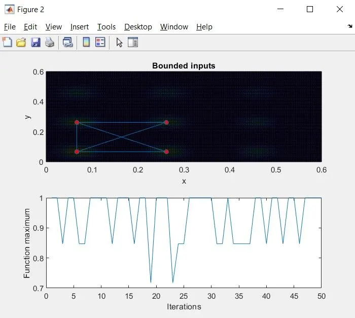
Here we can see that introducing the upper and lower bounds is giving better optimized values than earlier and there are just 2 values for x which are deviating from the result.

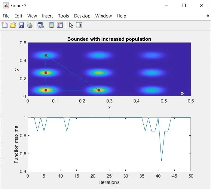
Again increasing the population has further optimized and gives a much closer result to the solution. Here we can see there is only one value deviating from the solution of the function and hence it is safe to say that the value obtained i.e., 0.8472 is the required maxima for the given stalagmite function.