Project 2 - Rankine cycle Simulator

Rankine Cycle:

The Rankine cycle is an idealized thermodynamic cycle of a heat engine that converts heat into mechanical work while undergoing phase change. It is an idealized cycle in which friction losses in each of the four components are neglected. The heat is supplied externally to a closed loop, which usually uses water as the working fluid.Water enters the pump at state 1 as saturated liquid and is compressed isentropically to the operating pressure of the boiler. The water temperature increases somewhat during this isentropic compression process due to a slight decrease inthe specific volume of water. Water enters the boiler as a compressed liquid at state 2 and leaves as a superheated vapor at state 3. The boiler is basically a large heat exchanger where the heat originating from combustion gases, nuclear reactors, or other sources is transferred to the water essentially at constant pressure. The boiler, together with the section where the steam is superheated, is often called the steam generator., The Rankine cycle closely describes the process by which steam-operated heat engines commonly found in thermal power generation plants generate power. Power depends on the temperature difference between a heat source and a cold source. The higher the difference, the more mechanical power can be efficiently extracted out of heat energy, as per Carnot's theorem. The heat sources used in these power plants are usually nuclear fission or the combustion of fossil fuels such as coal, natural gas, and oil, or concentrated solar power. The higher the temperature, the better. The efficiency of the Rankine cycle is limited by the high heat of vaporization of the working fluid.

Processes in a Rankine cycle:

process 1-2 ---> Isentropic expansion

process 2-3 ---> Isobaric heat rejection

process 3-4 ---> Isentropic compression

process 4-1 ---> Isobaric heat addition

Main Program:

% Rankine cycle Simulation
clear all
close all
clc

%Process description:
fprintf('1-2 Isentropic expansion\n')
fprintf('2-3 Isobaric heat rejection\n')
fprintf('3-4 Isentropic compression\n')
fprintf('4-1 Isobaric heat addition\n')

%Inputs from the user:
p1 = input('Enter the Pressure at the turbine inlet(in bar):');
t1 = input('Enter the temperature  at the inlet(in degree Celcius):');
p2 = input('Enter the Pressure at condenser(in bar):');

%Input conditions:
t = XSteam('Tsat_p',p1);
if t1>=t   %i.e., to check temp is greater than saturated temp,
    %Calculating state points
    h1 = XSteam('h_pt',p1,t1);
    s1 = XSteam('s_pt',p1,t1);
    
    %w.k.t s1 = s2 since it is isentropic expansion in the turbine
    s2 = s1;

    %getting the entropy values of liquid and gas with pressure data and 
    %then finding vapour fraction using the formulae s2= sf+x2*sfg
    sf2 = XSteam('sL_p',p2);
    sg2 = XSteam('sV_p',p2);
    x2 = (s2-sf2)/(sg2-sf2);
    
    %Getting the enthalpy values from the steam data w.r.t the pressure
    %and calculating the h2 value using h2 = hf2+x*(hg2-hf2)
    hf2 = XSteam('hL_p',p2);
    hg2 = XSteam('hV_p',p2);
    h2 = hf2 + x2*(hg2-hf2);
    
    %from rankine cycle diagram we have
    p3 = p2;
    p4 = p1;
    
    
         
    %For finding state points at point 3:
    h3 = XSteam('hL_p',p3);
    s3 = XSteam('sL_p',p3);
    t3 = XSteam('Tsat_p',p3);
    t2 = t3; %from rankine cycle diagram
    
    %calculating state points at point 4,5,6:
    s4 = s3;
    %Using the isentropic relations by getting the values of Cp and Cv:
    cp4 = XSteam('Cp_ps',p4,s4);
    cv4 = XSteam('Cv_ps',p4,s4);
    gamma = cp4/cv4;
    t4 = t3/((p3/p4)^((gamma-1)/gamma));
      
    h4 = XSteam('h_ps',p4,s4);
    t5 = XSteam('Tsat_p',p1);
    s5 = XSteam('sL_p',p1);
    s6 = XSteam('sV_p',p1);
    t6 = t5;
    
    % Plotting:
    temp = linspace(1,400,200);
for i = 1:length(temp)      %To draw the saturation line.
    ent_l(i) = XSteam('sL_T',temp(i));
    ent_v(i) = XSteam('sV_T',temp(i));
    enth_l(i) = XSteam('hL_T',temp(i));
    enth_v(i) = XSteam('hV_T',temp(i));
end

subplot(1,2,1)
plot([s1 s2 s3 s4 s5 s6 s1],[t1 t2 t3 t4 t5 t6 t1],'color','r','linewidth',3,'marker', 'o','markersize',2,'markerfacecolor','b')
hold on
plot(ent_l,temp,'color','b')
hold on
plot(ent_v,temp,'color','b')
hold on
axis([0 10 0 700])
text(s1,t1,'1','Fontsize',15)
text(s2,t2,'2','fontsize',15)
text(s3,t3,'3','fontsize',15)
text(s4,t4,'4','fontsize',15)
text(s5,t5,'5','fontsize',15)
text(s6,t6,'6','fontsize',15)
title('T-s diagram')
xlabel('Entropy')
ylabel('Temperature')
subplot(1,2,2)
plot([s1 s2 s3 s4 s1],[h1 h2 h3 h4 h1],'color','k','linewidth',3,'marker','o', 'markersize',2,'markerfacecolor','b')
axis([0 10 300 5000])
hold on
plot(ent_v,enth_v,'color','b')
plot(ent_l,enth_l,'color','b')
text(s1,h1,'1','fontsize',15)
text(s2,h2,'2','fontsize',15)
text(s3,h3,'3','fontsize',15)
text(s4,h4,'4','fontsize',15)
title('h-s diagram')
xlabel('Entropy')
ylabel('Enthalpy')

%RESULTS:
p = [p1 p2 p3 p4];
T = [t1 t2 t3 t4];
h = [h1 h2 h3 h4];
s = [s1 s2 s3 s4];
for j = 1:4     %Loop to print all four states values:
fprintf('At state point %d:\n',j);
fprintf('P%d is : %d\n',j,p(j));
fprintf('T%d is : %d\n',j,T(j));
fprintf('h%d is : %d\n',j,h(j));
fprintf('s%d is : %d\n\n',j,s(j));
end
fprintf('Wt is : %d\n',Wt);
fprintf('Wp is : %d\n',Wp);
fprintf('Wnet is : %d\n',Wnet);
fprintf('Ntherm is : %d\n',Ntherm);


else
fprintf('Enter temp greater or equal to saturation temperature\n');
end

The output screen is shown below:

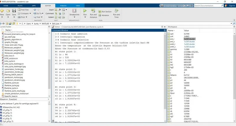
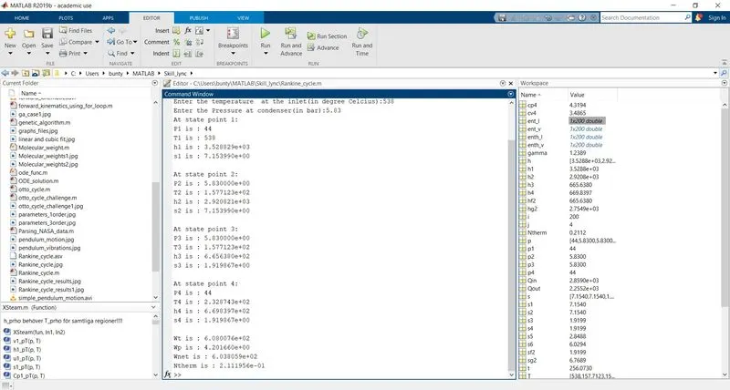
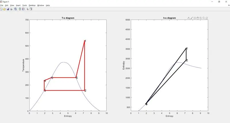
The plots of T-s and h-s are obtained as follows:

Conclusion:

Using the Xstream library data we can solve working cycles like rankine,carnot,reheat,regenerative cycle can be simulated with little effort on reading the values from the library Xstream.