Week 3 - Solving second order ODEs

Aim : To understand the motion of a simple pendulum using Matlab.

Theory:

A simple pendulum with mass 'm', length of string 'l', damping coefficient as 'b' is  considered with initial conditions given at time t=0 as angular displacment = 0 and angular velocity taken as 3 rads/sec.

A simple pendulum follows 2nd order differential equation given by 

`d theta^2/dt^2 + (b/m)*(d theta/dt) + (g/l)*sin theta = 0`

Procedure:

• First the ODE is broken to convert it into 1st order DE's. The DE's then obtained is as follows:`d (theta1)/dt = theta2` and`d (theta2)/dt = -(b/m)*theta2 - (g/l)*sin theta1`
• a solution equation in the form of matrix is obtained by the two equations which solve for angular displacement and angular velocity.

Code:

A code for defining the function ode_fun which gives the angular displacement and angular velocities as output is written first:

function [dtheta_dt] = ode_func(t,theta,b,g,l,m)
theta1 = theta(1)
theta2 = theta(2)
dtheta1_dt = theta2;
dtheta2_dt = -(b/m)*theta2 - (g/l)*sin(theta1);
[dtheta_dt] = [dtheta1_dt;dtheta2_dt];
end

Then the code for plotting the vibrations and also plotting the pendulum motion using the given inputs using the ode_fun function is written as follows:

%program for simple pendulum motion:
clear all
close all
clc

b=0.05;      %damping coefficient
g = 9.81;    %acceleration due to gravity in m/s^2
l=1;         %length of string in m
m=1;         %mass of the bob in kg
ct=1;        %counter variable 

% initial conditions:
theta_0 = [0;3];  %respective values of angular displacement and velocity are 
                  %initialized

%time points:
t_span = linspace(0,20,500);

%solving ODE using ode_func:
[t,results] = ode45(@(t,theta)ode_func(t,theta,b,g,l,m),t_span,theta_0);

figure(1)     %plotting the vibrations graph
hold on
plot(t,results(:,1))
plot(t,results(:,2))
ylabel('plot')
xlabel('time')
grid on 

figure(2)     %plotting the animation of pendulum

theta2 = results(:,1);   % the values of angular displacement calculated are stored in 
                         % theta2
for i = 1:length(theta2);
    theta_x = theta2(i);
    
    x0 = 0;
    y0 = 0;                 %fixing one end of the string
    x1 = l*sin(theta_x);
    y1 = -l*cos(theta_x);   %defining the position of other end of string
  
    plot([-1 1],[0 0],'linewidth',5,'color','b'); %plotting the fixed base where the 
                                                  %bob is suspended
    hold on
    plot([x0 x1],[y0 y1],'linewidth',2,'color','r') %plotting the string
    hold on
    plot(x1,y1,'o','markers',15,'markerfacecolor','y') % plotting a bob of defined 
                                                       % characteristics
    hold off
    grid on 
    axis([-1.5 1.5 -1.5 0.5]);   
    pause(0.002)
    M(ct) = getframe(gcf);  %function to dump all frames in 'M'
    ct = ct+1;

end
movie(M) Making a movie with all the images in M

videofile = VideoWriter('simple_pendulum_motion.avi','uncompressed AVI'); 
%defining the characteristics of the video file of animation created.

open(videofile)
writeVideo(videofile,M)
close(videofile)

Outputs:

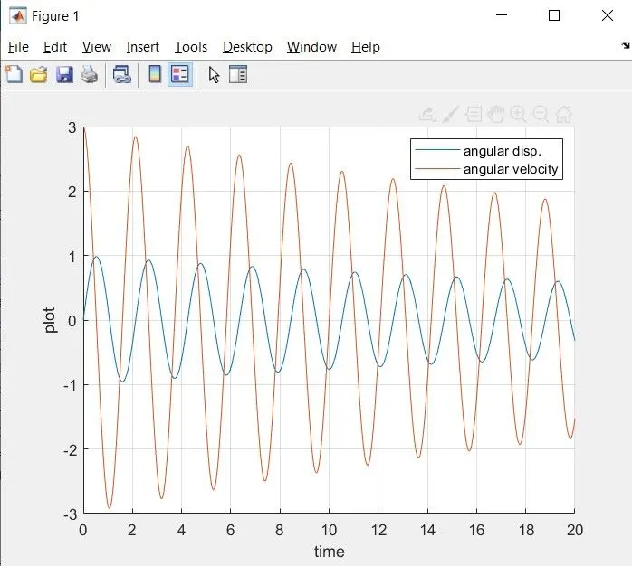
This is the graph showing angular displacements and angular velocities with respect to time.

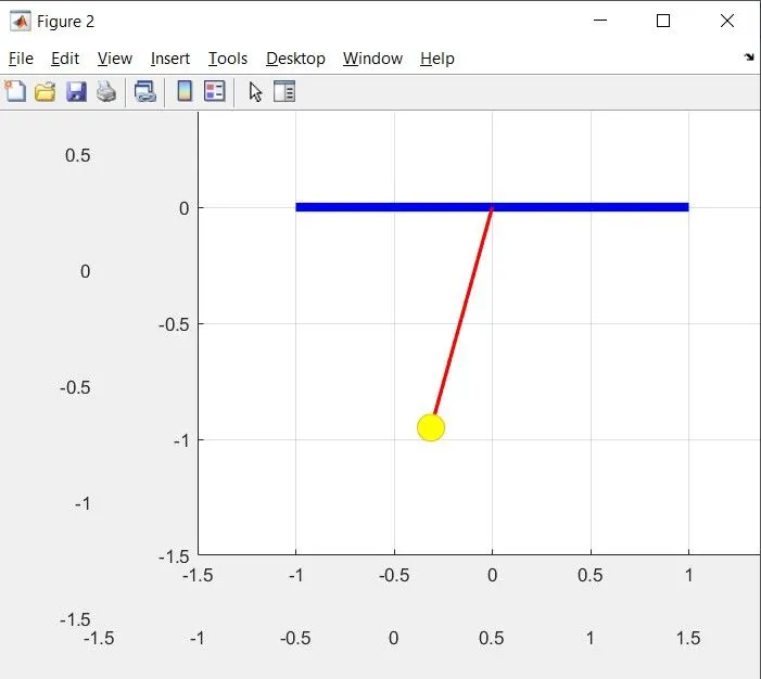
This is a snap from the pendulum motion plot.

The youtube link to the animation movie of the  motion of simple pendulum is shared below:

https://youtu.be/5KGbv4Y60MU