Week 4 - Genetic Algorithm

objective:

1) To write a code to optimise stalagmite function and find global maxima .

2) Explain the concept of genetic algorithm and explain the syntax for ga in MATLAB .

3) Ensure that the code gives consistent output over multiple runs .

4) Plot graphs for all the 3 cases and function max value vs number of iterations .

Theory :

Genetic algorithm is a search based optimization technique based on genetics and natural selection . It is frequently used to find optimum or near optimum solutions . It is used to solve non linear and non differential problems . It uses concepts from evolutionary biology .

Genetic algorithm a number of processes like selection , crossover and mutation to come up with near optimum solutions for a given function .

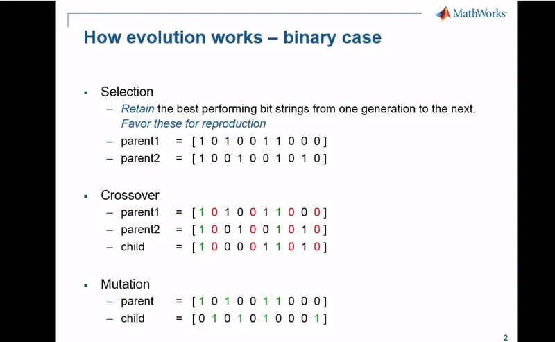
The fitness function then takes this as solution and compare with optimum values to check how close the solution is to the desired value .

Syntax for genetic algorithm

Genetic Algorithm has various syntaxes . Mentioned below are the brief description of syntaxes used in this particular program

1) x=ga(fun,nvar)

In the above syntax , x= solution

x= ga(fun,nvars) finds a local unconstrained minimum, x, to the objective function, fun.

nvars is the dimension (number of design variables) of fun

2) x = ga(fun,nvars,A,b,Aeq,beq,lb,ub)

x = ga(fun,nvars,A,b,Aeq,beq,lb,ub) defines a set of lower and upper bounds on the design variables, x, so that a solution is found in the range lb ≤ x ≤ ub. (Set Aeq=[] and beq=[] if no linear equalities exist.)

3)

x = ga(fun,nvars,A,b,Aeq,beq,lb,ub,nonlocon,options) minimizes with the default optimization parameters replaced by values in options. (Set nonlcon=[] if no nonlinear constraints exist.) Create options using optimoptions.

Program Logic :

a) Defining stalagmite function

function[Fxy] = stalagmite(input) : Defining [Fxy] as a function named stalgamite with an input (input)

x = input(1) : Defining x as an input (input1)
y = input(2) : Defining y as an input(input2)
f1x=(sin((5.1*pi*x)+0.5))^6 : Defining 1st part of given equation as a function of x
f1y= (sin((5.1*pi*y)+0.5))^6 : Defining 1st part of given equation as a function of y
f2x=exp(((-4*log(2))*((x-0.0667)^2 /0.64))) : Defining 2nd part of given equation as a function of x
f2y=exp(((-4*log(2))*((y-0.0667)^2 /0.64))) :Defining 2nd part of given equation as a function of y
n= (f1x*f1y*f2x*f2y) : Defining n as the stalagmite function equation
Fxy = -n : Applying negative value to obtain local maxima using ga

end : End of function definintion

b) Defining get_stalagmite function .

function[f]=get_stalagmite(x,y) : Defining a function (f) with name get_stalagmite with 2 variables x,y
x=linspace(0,0.6,150) : defiining x as an array with 150 values between 0 and 0.6
y=linspace(0,0.6,150) : defiining y as an array with 150 values between 0 and 0.6

[xx yy]=meshgrid(x,y) : command to make the array [xx yy] into a 2D meshgrid .

for i= 1:length(xx) : opening 1st for loop to vary value of i according to number of array xx
for j=1:length(yy) :opening 2nd for loop to vary value of j according to number of array yy

input_vector(1)=xx(i,j) : Defining input_vector 1 as array xx(i,j)
input_vector(2)=yy(i,j) : Defining input_vector 2 as array yy(i,j)
f(i,j)=(stalagmite(input_vector)) : callling stalagmite function with variables x and y

end : end of 2nd for loop
end : end of first for loop
end : end of function definition

c) Main program

clear all
close all
clc

x=linspace(0,0.6,150) : Defining an array x with 150 values from 0 to 0.6

y=linspace(0,0.6,150) : Defining an array y with 150 values from 0 to 0.6
num_cases=50 : Defining the number of cases for for loop .
f=get_stalagmite(x,y) : calling stalagmite function defined above with variables x,y

Study1 - statistical behaviour wihtout constraints
tic : defining tic to call toc later to obtain run time .
for i=1:num_cases : initiating for loop with i = number of cases

[inputs,fopt(i)]=ga(@stalagmite,2) : calling genetic algorithm with stalagmite function defined earlier
xopt(i)=inputs(1) : defining x optimum as output column 1 from ga
yopt(i)=inputs(2) : defining y optimum as output column 2 from ga

end : End of for loop

figure(1)
subplot(2,1,1) : command to divide plot to 2 rows and 1 column and 1st position
hold on : command to hold on to plot
surfc(x,y,-f) : command to create surface plot with values x,y and negative f
title('Unconstrained Plot') : command to create title for plot as unconstrained plot
xlabel('X-axis') : command to label x axis as x axis
ylabel('y-axis') : command to label y axis as y axis
zlabel('value of function') : command to label z axis as value of function
shading interp : command to remove mesh grid representation
plot3(xopt,yopt,-fopt,'marker','o','markersize',5,'markerfacecolor','r') : command to create marker with size 5 and color red
subplot(2,1,2) : command to define plot wiht 2 rows,1 column and 2nd plot
plot(-fopt) : command to plot 2nd plot with value of f optimum
xlabel('Iterations') :command to label x axis as iterations
ylabel('Function maximum') :command to label y axis as function maximum
study1_time=toc : command to obtain runtime for case 1 using toc

Study2- statistical behaviour with upper and lower bounds
tic :defining tic to call toc later to obtain run time .
for i=1:num_cases : initiating for loop with i = number of cases

[inputs_b,fopt_b(i)]=ga(@stalagmite,2,[],[],[],[],[0;0],[0.6;0.6]) :calling genetic algorithm with stalagmite function defined earlier by defining upper and lower bounds for x and y as 0 and 0.6

xopt_b(i)=inputs_b(1) :defining x optimum as output column1 from ga
yopt_b(i)=inputs_b(2) :defining y optimum as output column2 from ga

end : End of for loop

figure(2) : to create new figure2
subplot(2,1,1) : command to divide plot to 2 rows and 1 column and 1st position
hold on :command to hold on to plot
surfc(x,y,-f) :command to create surface plot with values x,y and negative f
shading interp : command to remove mesh grid representation
title('Constrained Plot') :command to create title for plot as constrained plot
xlabel('X-axis') : command to label x axis as x axis
ylabel('y-axis') :command to label y axis as y axis
zlabel('value of function') : command to label z axis as value of function
plot3(xopt_b,yopt_b,-fopt_b,'marker','o','markersize',5,'markerfacecolor','r') : command to create a plot with x optimum,yoptimum and f optimum and circle marker with size 5 and color red
subplot(2,1,2) :command to define plot with 2 rows,1 column and 2nd plot
plot(-fopt_b) :command to plot 2nd plot with value of f optimum
xlabel('Iterations') :command to label x axis as iterations
ylabel('Function maximum') :command to label y axis as function maximum
study2_time=toc :command to obtain runtime of study 2 with toc

Study3 - Increasing GA iterations

options=optimoptions('ga') : to return set of default values for solver ga
options=optimoptions(options,'populationsize',200) : to vary the default value of population size in ga to 200

tic :defining tic to call toc later to obtain run time .
for i=1:num_cases : initiating for loop with i = number of cases

[inputs_c,fopt_c(i)]=ga(@stalagmite,2,[],[],[],[],[0;0],[0.6;0.6],[],[],options) :calling genetic algorithm slover with upper bounds , lower bounds and varied iteration values

xopt_c(i)=inputs_c(1) :defining x optimum as ouput column1 from ga
yopt_c(i)=inputs_c(2) :defining y optimum as output column2 from ga

end : End of for loop

figure(3) : command to create a new figure
subplot(2,1,1) : command to divide plot to 2 rows and 1 column and 1st position
hold on :command to hold on to plot
surfc(x,y,-f) :command to create surface plot with values x,y and negative f
title('Constrained Plot with increased iterations') :command to create title for plot
xlabel('X-axis') : command to label x axis as x axis
ylabel('y-axis') :command to label y axis as y axis
zlabel('value of function') :command to label z axis as value of function
shading interp : command to remove mesh grid representation

plot3(xopt_c,yopt_c,-fopt_c,'marker','o','markersize',5,'markerfacecolor','r') : command to create a plot with xoptimum,yoptimum and f optimum and a circle marker with size 5 and color red

subplot(2,1,2) :command to define plot with 2 rows,1 column and 2nd plot
plot(-fopt_c) :command to plot 2nd plot with value of f optimum
xlabel('Iterations') :command to label x axis as iterations
ylabel('Function maximum') :command to label y axis as function maximum
study3_time=toc :command to obtain runtime of study using toc

Code:

1) Stalagmite function

function[Fxy] = stalagmite(input)
        
x = input(1)
y = input(2)
f1x=(sin((5.1*pi*x)+0.5))^6;
f1y= (sin((5.1*pi*y)+0.5))^6;
f2x=exp(((-4*log(2))*((x-0.0667)^2 /0.64)));
f2y=exp(((-4*log(2))*((y-0.0667)^2 /0.64)));
n= (f1x*f1y*f2x*f2y);
Fxy = -n;

end

   

2) get_stalagmite function

function[f]=get_stalagmite(x,y)
  x=linspace(0,0.6,150);
   y=linspace(0,0.6,150);


[xx yy]=meshgrid(x,y);


for i= 1:length(xx)
    for j=1:length(yy)
        
        input_vector(1)=xx(i,j);
        input_vector(2)=yy(i,j);
        f(i,j)=(stalagmite(input_vector));
        
    end
end
end

3)

Main program

clear all 
close all 
clc

x=linspace(0,0.6,150);
y=linspace(0,0.6,150);
num_cases=50
f=get_stalagmite(x,y);

% Study1 - statistical behaviour wihtout constraints
tic
for i=1:num_cases 
   
    [inputs,fopt(i)]=ga(@stalagmite,2);
        xopt(i)=inputs(1);
        yopt(i)=inputs(2);
        
end

figure(1)
subplot(2,1,1)
hold on
surfc(x,y,-f)
title('Unconstrained Plot')
xlabel('X-axis')
ylabel('y-axis')
zlabel('value of function')
shading interp
plot3(xopt,yopt,-fopt,'marker','o','markersize',5,'markerfacecolor','r')
subplot(2,1,2)
plot(-fopt)
xlabel('Iterations')
ylabel('Function maximum')
study1_time=toc


%Study2- statistical behaviour with upper and lower bounds
tic
for i=1:num_cases 
   
    [inputs_b,fopt_b(i)]=ga(@stalagmite,2,[],[],[],[],[0;0],[0.6;0.6]);
        xopt_b(i)=inputs_b(1);
        yopt_b(i)=inputs_b(2);
        
end

figure(2)
subplot(2,1,1)
hold on
surfc(x,y,-f)
shading interp
title('Constrained Plot')
xlabel('X-axis')
ylabel('y-axis')
zlabel('value of function')
plot3(xopt_b,yopt_b,-fopt_b,'marker','o','markersize',5,'markerfacecolor','r')
subplot(2,1,2)
plot(-fopt_b)
xlabel('Iterations')
ylabel('Function maximum')
study2_time=toc

%study3 - Increasing GA iterations
options=optimoptions('ga');
options=optimoptions(options,'populationsize',200);

tic
for i=1:num_cases 
   
    [inputs_c,fopt_c(i)]=ga(@stalagmite,2,[],[],[],[],[0;0],[0.6;0.6],[],[],options);
        xopt_c(i)=inputs_c(1);
        yopt_c(i)=inputs_c(2);
        
end

figure(3)
subplot(2,1,1)
hold on
surfc(x,y,-f)
title('Constrained Plot with increased iterations')
xlabel('X-axis')
ylabel('y-axis')
zlabel('value of function')
shading interp

plot3(xopt_c,yopt_c,-fopt_c,'marker','o','markersize',5,'markerfacecolor','r')
subplot(2,1,2)
plot(-fopt_c)
xlabel('Iterations')
ylabel('Function maximum')
study3_time=toc

Results :

case1

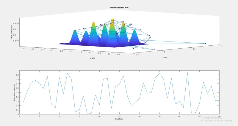
Here we can observe that the ga produces varying values all over the range . The optimisation is minimum in this case as there are no constrains .

case 2 :

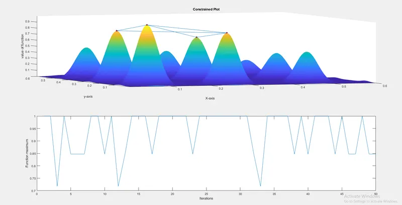
In this case , we observe that the optimisation has improved a lot and the obtained values fall between 0.6 and 0.9 . This is because of the introduction of constrains .

case3:

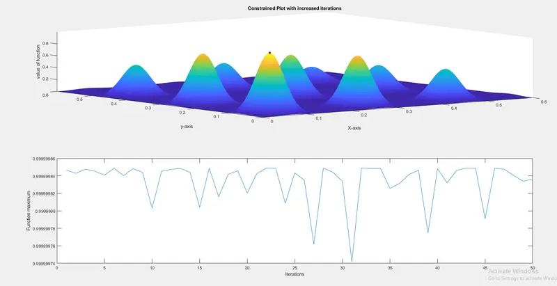
In this case , we observe that the optimisation has been maximized and we get almost constant optimisation output . This is because of the increased number of iterations and constrains .

Hence the global maximum value has been optimised .

Errors occured :

1)

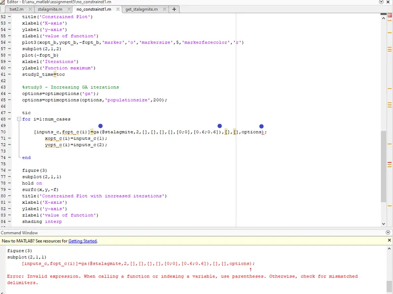
This error occured dueto an extra closing bracket in the command . All 3 brackets are denoted by a blue dot above them .

2)

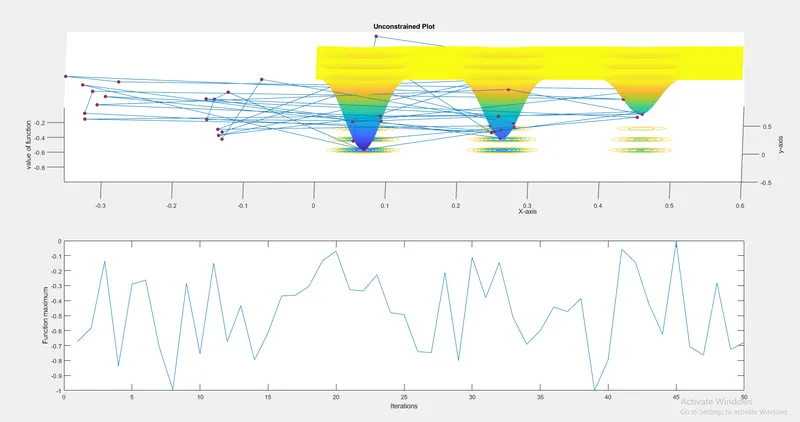
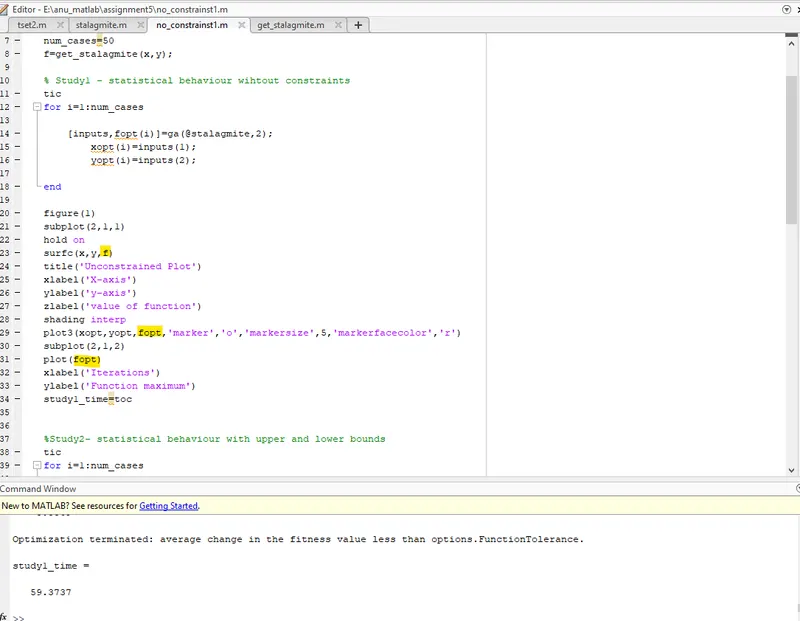
This was not an error , however this solution found was global minima instead of global maxima . Hence the value of f , while being plotted was changed to negative inorder to obtain maximum values for f . Hence the issue was resolved. The points in which f was negated have been highlighted by yellow marker .