Week 4 - Genetic Algorithm
AIM: To execute a code in MATLAB to optimise the stalagmite function and find the global maxima of the function.
Introduction to Geneitc algorithm:
Genetic Algorithm: It is a search baesd optimization technique which is based on the principled of genetic and natural selection. It will help to find the optimal and near optimal solutions in which the problems will took a lifetime to solve. genetic algorithm is based on the theory of CHARLES DARWIN THEORY OF NATURAL SELECTION. We have to select randomly for better output and input parameters has to be optimal in order to find input values , genetic algorithm plays a major role.
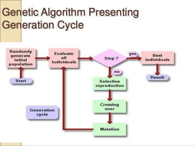
Genetic algorithm is classified as shown below,
1.Selection
2.Cross-Over
3.Mutation
1.Selection:
It selects the individuals from the present population called parents that contribut at the next generation. We should select the individual and allow them to create their offsprings. But it would lead to individuals that are more close to one another in a few next generation, and therefore less diversity. In this selection process, we generally use Roulette Wheel Selection method.
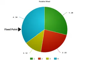
iIn this method, the individuals are divided into 4 number of divisions as per the population. The percentage of the every individual is shown in different colurs that could be easy to find ourselves.So, now this wheel is rotated and the region of wheel which comes in front of the fixed point is chosen as the parent.
2.Cross-Over:
In this previous step, we have selected parent individuals that will produce off-springs. So in biological terms, crossover is nothing but reproduction.Now we have to find the crossover of chromosome 1 and 4, which were selected in the previous step. Take a look at the image below.
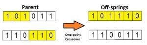
This is the most basic form of crossover, known as one point crossover. Here we select a random crossover point and the tails of both the chromosomes are swapped to produce a new off-springs.
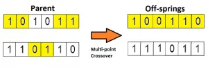
If you take two crossover point, then it will called as multi point crossover which is as shown below.
3.Mutation:
It is defined as a random tweak in the chromosome, which also promotes the idea of diversity in the population. A simple method of mutation is shown in the image below.

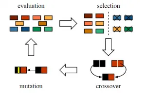
So the entire process is shown in the figure.The off-springs thus produced are again validated using our fitness function, and if considered fit then will replace the less fit chromosomes from the population.
Syntax for ga:
- x = ga(fun,nvars). It finds a local unconstrained minimum, x, to the objective function, fun. nvars is the dimension (number of design variables) of fun.
x = ga(fun,nvars,A,b). It finds a local minimum x to fun, subject to the linear inequalities A*x ≤ b.ga evaluates the matrix product A*x as if x is transposed (A*x').x = ga(fun,navrs,A,b,Aeq,beq). It finds a local minimum x to fun, subject to the linear equalities Aeq*x = beq and A*x ≤ b. (Set A=[] and b=[] if no linear inequalities exist.) ga evaluates the matrix product Aeq*x as if x is transposed (Aeq*x').x = ga(fun,nvars,A,b,Aeq,beq,lb,ub). It defines a set of lower and upper bounds on the design variables, x, so that a solution is found in the range lb ≤ x ≤ ub. (Set Aeq=[] and beq=[] if no linear equalities exist.)x = ga(fun,nvars,A,b,Aeq,beq,lb,ub,nonlcon). It subjects the minimization to the constraints defined in nonlcon. The function nonlcon accepts x and returns vectors C and Ceq, representing the nonlinear inequalities and equalities respectively. ga minimizes the fun such that C(x) ≤ 0 and Ceq(x) = 0. (Set lb=[] and ub=[] if no bounds exist.)x = ga(fun,nvars,A,b,Aeq,beq,lb,ub,nonlcon,options).It minimizes with the default optimization parameters replaced by values in options. (Set nonlcon=[] if no nonlinear constraints exist.)x = ga(fun,nvars,A,b,[],[],lb,ub,nonlcon,IntCon)or x = ga(fun,nvars,A,b,[],[],lb,ub,nonlcon,IntCon,options).It requires that the variables listed in IntCon take integer values.x = ga(problem).It finds the minimum for problem, a structure described in problem.[x,favl] = ga(___), for any previous input arguments, also returns fval, the value of the fitness function at x.[x,fval,exitflag,output] = ga(___). It also returns exitflag, an integer identifying the reason the algorithm terminated, and output, a structure that contains output from each generation and other information about the performance of the algorithm.[x,fval,exitflag,output,population,scores] = ga(___). It also returns a matrix population, whose rows are the final population, and a vector scores, the scores of the final population.
where
- x = ga(fun,nvars,A,b,[],[],lb,ub,nonlcon,IntCon,options)
- fun - fitnesss function.
- nvars - Number of design variables.
- A [] = A matrix for linear inequality constraints.
- b [] = b vector for linear inequality constraints.
- Aeq [] = Aeq matrix for linear equality constraints.
- beq [] = beq vector for linear equality constraints.
- lb = lower bound on x.
- ub = upper bound on x.
- nonlcon [] = non linear constraint function.
- Intcon [] = interger constraint function.
- options - Options created using optimoptions or an options structure
Objective:
- To write a code to optimize the stalagmite function and to find the global maxima of it by using matlab software.
- Expalin the concept of genetic algorithm and also explain the syntax for ga in MATLAB.
- Plot graphs for all 3 studies and for F maximum vs no. of iterations. Title and axes labels are a must, legends could be shown if necessary.
Prcoedure:
- First we have to define the stalagmite function in the separetey.
- In the stalagmite fuction, we have to give negative sign for the equation because the function is used to obtain the maxima but not minima.
- For loop is used to iterate the each of the elements in all the three conditions.
- Genetic algorithm is used to obtain the optimal value of the function.
The plot is generated for the three different cases are shown below.
- Unbounded inputs.
- Bounded inputs - restrictions with upper and lower bounds.
- Bounded inputs - increasing number of iterations by giving population size.
Explanation and Program code by using Matlab Software:
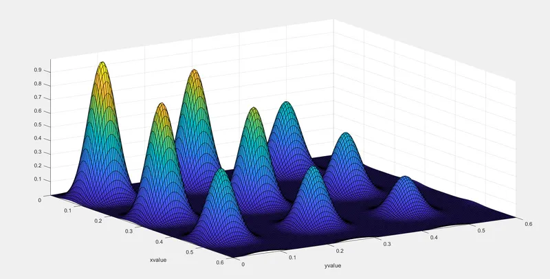
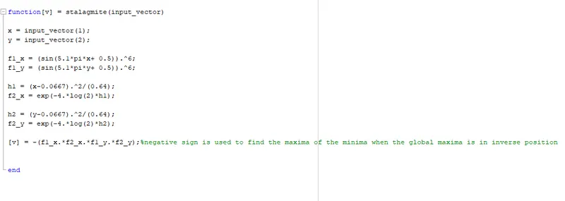
The stalagmite fuction is shown in the image form and in the form of code.
function[v] = stalagmite(input_vector)

x = input_vector(1);
y = input_vector(2);

f1_x = (sin(5.1*pi*x+ 0.5)).^6;
f1_y = (sin(5.1*pi*y+ 0.5)).^6;

h1 = (x-0.0667).^2/(0.64);
f2_x = exp(-4.*log(2)*h1);

h2 = (y-0.0667).^2/(0.64);
f2_y = exp(-4.*log(2)*h2);

[v] = -(f1_x.*f2_x.*f1_y.*f2_y);

end
- First a variable 'v' is defined for the slagmite function.
- Stalagmite function takes the values of 'input vector' and calculates the value of 'v'.
- The function 'v' calculates the values of two variables (x ,y).
- The terms involved in the formula are [f1_x, f2_x, f1_y, f2_y].
- x is stored in an array called 'input vector(1)'.
- y is stored in an array called 'input vector(2)'.
- And all the term are multiplied and a '-' sign is given in the syntax to make the plot in positive x-axis.
The program is shown for finding the three different cases of iterations as shown in figure.
close all                                          %to clear all the previous running fuctions in the workspace
clear all                                          %to close all the previous plots & graphs running in the background
clc                                                %to clear the workspace
%defining our search space
x = linspace(0,0.6,150);                           %specify the x-axis to plot the graph from 0-0.6
y = linspace(0,0.6,150);                           %specify the y-axis to plot the graph from 0-0.6

%creating a 2Dimensional mesh
[xx yy] = meshgrid(x,y);                          % it returns 2D grid coordinates contained in the vector x and y

%evaluating the stalagmite function
for i =1:length (xx);                               % to define a values for the whole length of x
         for j = 1:length(yy);                      % to define a values for the whole length of y
             input_vector(1) = xx(i,j);             % input vector is a row vector it has two columns.
             input_vector(2) = yy(i,j);             % values of x and Y assigned in array called as input vector.
             f(i,j) = stalagmite(input_vector);    % the stalagmite function named in input vector, it called as function.
         end
end

[inputs,fval] = ga(@stalagmite,2)
shading interp                    % to disable the shading command in the graph
surfc(x,y,f)
xlabel('xvalue')
ylabel('yvalue')
- clear all - Clear all command is used to clear all the previous running function in the workspace.
- close all - Close all command is used to close all the previous running plots and graphs running in the background.
- clc - clc command is used to clear the workspace.
- Then we use the 'meshgrid' command.
- 'i' is a variable used to define the values for the whole length of x.
- 'j' is a variable used to define the values for the whole length of y.
- 'input_vector' is a row vector i.e it has 2 columns.
- We take the two values of x and y and put them in an array called the 'input_vector'.
- Now the function stalagmite takes in the input vector and calculates the value of 'f'.
- 'end' command is used to finish the for loop.
- Then we have to call the stalagmite function with two variables as '2' and assigning it as genetic algorithm.
- '[inputs, fopt(i)]' - calculates the optimum value of 'f' for the specific range of the function.
- Shading command is used to disable the shading over the graph.
- xlabel is the command which names the label on the x-axis as x value.
- ylabel is the command which names the label on the y-axis as y value.
Plot:
The plot which is about stalagmite function as shown in figure.
Case-1: Unbounded conditions :-
%study-1 statistical behaviour
%UNBOUNDED CONDITIONS

tic                                                   %tic_toc command for iteeration time
for i =1:num_cases
    [inputs, fopt(i)] = ga(@stalagmite,2);
    xopt(i) = inputs(1);
    yopt(i) = inputs(2);
end

study_1_time = toc;
figure(1)
subplot(2,1,1)
hold on
surfc(x,y,-f)
shading interp
plot3(xopt,yopt,-fopt,'marker','o','markersize',5,'markerfacecolor','r')
title('Unbounded inputs')
xlabel('x axis')
ylabel('y axis')
grid on
subplot(2,1,2)
plot(-fopt)
xlabel('iterations')
ylabel('function minimum value')
Explanation of code :
- We use the tic and toc command to calculate the study time.
- 'tic' function works with the 'toc' function to measure the elapsed time.
- The 'tic' function records the current time, and the 'toc' function uses the recorded value to calculate the elapsed time.
- The command 'num_cases' instructs the matlab to run the function for 50 iterations and evaluate the fitness value of the function.
- Then we create a 'for loop' with a variable 'i'.
- 'i = 1:num_cases' - is a command which stores the values for each 50 iterations of fitness for this function.
- '[inputs, fopt(i)]' - calculates the optimum value of 'f' for the specific range of the function.
- 'stalagmite' - is the command which is used to call the stalagmite function which we have saved to make the coding easier.
- xopt(i) assigns the input for first variable.
- yopt(i) assigns the input for second variable.
- We use 'end' command to close the 'for' loop.
Plot:
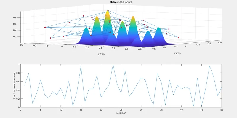
Explanation of plotting the graph:
- We use subplot command,for the figure(1).
- 'subplot(2,1,1)' divides the current figure into an 2-by-1 grid and creates axes in the specified position by 1. If axes exist in the specified position, then this command makes the axes as the current axes.
- 'surfc(X,Y, f)' creates a three-dimensional surface plot, which is a three-dimensional surface that has solid edge colors and solid face colors.
- The function plots the values in matrix 'f' as heights above a grid in the X-Y plane defined by xx and yy. The color of the surface varies according to the heights specified by f.
- 'hold on' command is used to hold both the plots.
- Here, we use the 'plot3' command to make the 3-D array of (xopt,yopy,-fopt), with a marker 'o' markersize 5 and color red.
- The '-' sign is given to make the plot on a positive x- axis, for our own convenience.
- xlabel is the command which names the label on the x-axis.
- ylabel is the command which names the label on the y-axis.
- 'plot(-fopt)' plots the graph for the different value of the fitness of the stalagmite function.
- 'xlabel' is the command which names the label on the x-axis as 'Iterations'.
- 'ylabel' is the command which names the label on the y-axis as 'Function minimum value'.
Result for plot1:
- study time for study-1 (unbounded conditions)is 4.897.
- But the plot and hence the optimization is not accurate.
Case-2: Bounded conditions with lower and upper bounds:-
%STUDY-2 BOUNDED CONDITION

tic                                   %tic_toc command for calculating the iteration time
for i =1:num_cases;
    [inputs,fopt(i)] = ga(@stalagmite,2,[],[],[],[],[0;0],[0.6;0.6]);
     xopt(i) = inputs(1);
     yopt(i) = inputs(2);
end
 study_2_time = toc
 %plotting the grapgh
 figure(2)
 subplot(2, 1, 1)
 hold on
 surfc(x,y,-f)
 plot3(xopt,yopt,-fopt,'marker','o','markersize',5,'markerfacecolor','r')
 xlabel('x axis')
 ylabel('y axis')
 title('Bounded inputs')
 subplot(2,1,2)
 plot(-fopt)
 xlabel('Iteration')
 ylabel('Function minimum value')
Explanation of code:
- We use the tic and toc command,to calculate the study time.
- 'tic' works with the 'toc' function to measure elapsed time.
- The 'tic' function records the current time, and the 'toc' function uses the recorded value to calculate the elapsed time.
- The command 'num_cases' instructs the matlab to run the function for 50 iterations and evaluate the fitness.
- Then we create a 'for loop' with a variable 'i'.
- 'i= 1:num_cases' - is the variable command which stores the values for each 50 iteration of fitness for this function.
- '[inputs, fopt(i)]' - calculates the optimum value of 'f' for the specific range of the function.
- 'stalagmite' - is the command which is used to call the stalagmite function which we have saved to make the coding easier.
- xopt(i) takes the input for 1st variable.
- yopt(i) takes the input for 2nd variable.
- we use 'end' command to close the for loop.
Plot:
Explanation of plot:
- We use subplot command,for the figure(2).
- 'subplot(2,1,1)' divides the current figure into an 2-by-1 grid and creates axes in the position specified by 1.
- If axes exist in the specified position, then this command makes the axes the current axes.
- 'surf(X,Y, f)' creates a three-dimensional surface plot, which is a three-dimensional surface that has solid edge colors and solid face colors.
- The function plots the values in matrix 'f' as heights above a grid in the X-Y plane defined by xx and yy. The color of the surface varies according to the heights specified by f.
- 'hold on' command is used to keep both the plots.
- Here, we use the 'plot3' command to make the 3-D array of (xopt,yopy,-fopt), with a marker 'o' markersize 5 and color red.
- The '-' sign is given to make the plot on a positive x- axis, for our own convenience.
- 'xlabel' is the command which is named as x-axis.
- 'ylabel' is the command which is named as y-axis.
- 'plot(-fopt)' plots the graph for the different value of the fitness of the stalagmite function.
- 'xlabel' is the command which is labelled as 'Iterations'.
- 'ylabel' is the command which is labelled as 'Function minimum value'.
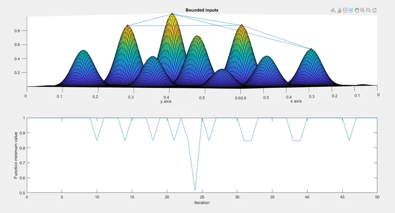
Result for study time-2:
- The study time is for the study time -2(bounded conditions) is 3.2589
- By observing the plot, we can understood that by giving a boundary condition the optimization is more accurate and variation decreased to countable numbers of plots.
- But,we need to specify a population size to the study for accurate and better result.
Case-3: study with increase in population size:-
%study-3  |increasing with population size

options = optimoptions('ga');                                      %calcualating the optimum solution for ga and save in options(variable)
 options = optimoptions(options,'PopulationSize',240);              %increasing the size of population

 tic                                   %tic_toc command for iteeration time
 for i= 1:num_cases
     [inputs,fopt(i)] = ga(@stalagmite,2,[],[],[],[],[0;0],[0.6;0.6],[],[],options);
       xopt(i) = inputs(1);
       yopt(i) = inputs(2);

 end
study_3_time = toc

%plotting the graph
figure(3)
subplot(2,1,1)
hold on
surfc(x,y,-f)
shading interp
plot3(xopt,yopt,-fopt,'marker','o','markersize',5,'markerfacecolor','r')
xlabel('x axis')
ylabel('y axis')
title('increase in population')
subplot(2,1,2)
plot(-fopt)
xlabel('Iteration')
ylabel('Function minimum value')
Explanation of code:
- We use the tic and toc command to calculate the study time.
- 'tic' function works with the 'toc' function to measure the elapsed time. The 'tic' function records the current time, and the 'toc' function uses the recorded value to calculate the elapsed time.
- The command 'num_cases' instructs the matlab to run the function for 50 iterations and evaluate the fitness value.
- Then we create a 'for loop' with a variable 'i'.
- i= 1:num_cases- is the variable command which stores the values for each 50 iteration of fitness for this function.
- '[inputs, fopt(i)]' - calculates the optimum value of 'f' for the specific range of the function.
- 'stalagmite' - is the command which is used to call the stalagmite function which we have saved to make the coding easier.
- xopt(i) takes the input for 1st variable.
- yopt(i) takes the input for 2nd variable.
- we 'end' the for loop.
Plot :
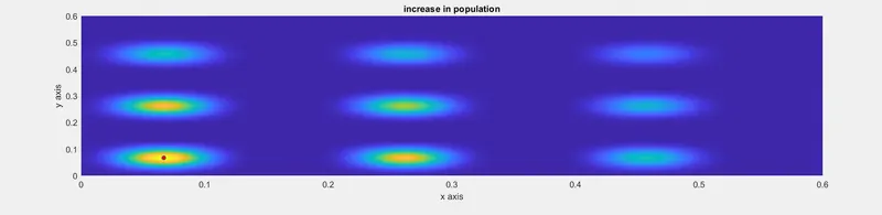
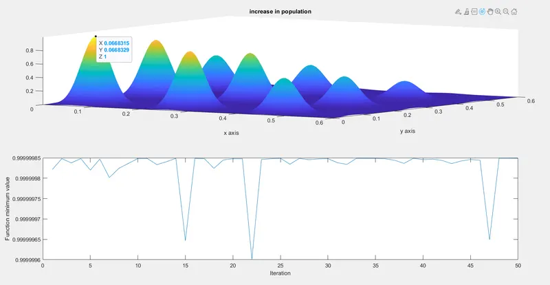
Plot:
- We use subplot command,for the figure(3).
- 'subplot(2,1,1)' divides the current figure into an 2-by-1 grid and creates axes in the position specified by 1.
- If axes exist in the specified position, then this command makes the axes the current axes.
- 'surfc(x,y,-f)' creates a three-dimensional surface plot, which is a three-dimensional surface that has solid edge colors and solid face colors.
- The function plots the values in matrix 'f' as heights above a grid in the X-Y plane defined by xx and yy. The color of the surface varies according to the heights specified by f.
- 'hold on' command is used to keep both the plots.
- Then,we use the 'plot3' command to make the 3-D array of (xopt,yopy,-fopt), with a marker 'o' markersize 5 and color red.
- The '-' sign is given to make the plot on a positive x- axis, for our own convenience.
- 'xlabel' is the command which is named as x-axis.
- 'ylabel' is the command which is named as y-axis.
- 'plot(-fopt)' plots the graph for the different value of the fitness of the stalagmite function.
- xlabel is given the name 'Iterations'.
- ylabel is given the name 'Function minimum value'.
Result for Study time-3:
- By increasing the population size,the optimal value is shown at the global maxima at 240.
- The study time for study-3(increasinfg with population size) is 9.8507
- The optimal value for x is x = 0.0668315.
- The optimal value for y is y = 0.0668329
- The value of f = 1,which is absolute value for optimal solution.
Matlab program code :
close all
clear all
clc
%defining our search space
x = linspace(0,0.6,150);
y = linspace(0,0.6,150);
num_cases = 50                                      %ga is going to run for 50 times

%creating a 2Dimensional mesh
[xx yy] = meshgrid(x,y);                          % it returns 2D grid coordinates contained in the vector x and y


%evaluating the stalagmite function
for i = 1:length (xx);                               % to define a values for the whole length of x
         for j = 1:length(yy);                       % to define a values for the whole length of y
             input_vector(1) = xx(i,j);              % input vector is a row vector it has two columns.
             input_vector(2) = yy(i,j);              % values of x and Y assigned in array called as input vector.
             input_vector = [input_vector(1),input_vector(2)];
             f(i,j) = stalagmite(input_vector);      % the stalagmite function named in input vector, it called as function.
         end
end


%study-1 statistical behaviour
%UNBOUNDED CONDITIONS
tic                                               %tic_toc command to study the iteration time
for i =1:num_cases
    [inputs, fopt(i)] = ga(@stalagmite,2);
    xopt(i) = inputs(1);
    yopt(i) = inputs(2);
end

study_1_time = toc
figure(1)
subplot(2,1,1)
hold on
surfc(x,y,-f)
shading interp
plot3(xopt,yopt,-fopt,'marker','o','markersize',5,'markerfacecolor','r')
title('Unbounded inputs')
xlabel('x axis')
ylabel('y axis')
subplot(2,1,2)
plot(-fopt)
xlabel('iterations')
ylabel('function minimum value')

%STUDY-2 BOUNDED CONDITION

tic                                   %tic_toc command for calculating the iteration time
for i =1:num_cases;
    [inputs,fopt(i)] = ga(@stalagmite,2,[],[],[],[],[0;0],[0.6;0.6]);
     xopt(i) = inputs(1);
     yopt(i) = inputs(2);
end
 study_2_time = toc
 %plotting the grapgh
 figure(2)
 subplot(2, 1, 1)
 hold on
 surfc(x,y,-f)
 plot3(xopt,yopt,-fopt,'marker','o','markersize',5,'markerfacecolor','r')
 xlabel('x axis')
 ylabel('y axis')
 title('Bounded inputs')
 subplot(2,1,2)
 plot(-fopt)
 xlabel('Iteration')
 ylabel('Function minimum value')

 %study-3  |increasing with population size

 options = optimoptions('ga');                                      %calcualating the optimum solution for ga and save in options(variable)
 options = optimoptions(options,'PopulationSize',240);              %increasing the size of population

 tic                                   %tic_toc command for iteeration time
 for i= 1:num_cases
     [inputs,fopt(i)] = ga(@stalagmite,2,[],[],[],[],[0;0],[0.6;0.6],[],[],options);
       xopt(i) = inputs(1);
       yopt(i) = inputs(2);

 end
study_3_time = toc

%plotting the graph
figure(3)
subplot(2,1,1)
hold on
surfc(x,y,-f)
shading interp
plot3(xopt,yopt,-fopt,'marker','o','markersize',5,'markerfacecolor','r')
xlabel('x axis')
ylabel('y axis')
title('increase in population')
subplot(2,1,2)
plot(-fopt)
xlabel('Iteration')
ylabel('Function minimum value')
Error in the code:
Error-1:
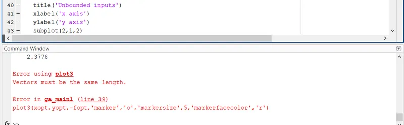
The above error was corrected by giving the input for fopt(i) in the syntax which we had given in study-3.
[inputs, fopt(i)] = ga(@stalagmite,2,[],[],[],[],[0;0],[0.6;0.6],[],[],options)The marker should not be given by our own. There are some strings to specify the marker like 'diamond', 'o', etc.
Error-2:
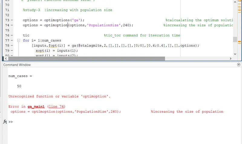
The error which is shown above is, we have to mention the spell the 'optimoptions' correctly.
Error-3:
We have to mention the elemental operators correctly and expressing way for the function is also taken into account while runnningthe function.
References:
- https://skill-lync.com/knowledgebase/genetic-algorithm-explained
- https://www.tutorialspoint.com/genetic_algorithms/genetic_algorithms_introduction.htm
- The document present in matlab software called 'doc ga'.Syntax about genetic algorithm is explained clearly.