Week 3 - Solving second order ODEs

Aim:Write a program in Matlab that will simulate the pendulum motion and animate the motion of the pendulum through ode function.

The equation of motion of a simple pendulum with damping is given by,

The values given are,

g = gravity = 9.81 m/s2.

L = length of the pendulum= 1 metre.

m = mass of the ball= 1 kg,

b=damping coefficient = 0.05.

Objective : To simulate the pendulum motion between 0-20 sec, for angular displacement=0,angular velocity=3 rad/sec at time t=0.

To write a program by using Matlab software to obtain an animation of the motion of the pendulum by using an ode function.

Matlab programs with ODE functions:

The functions below used in the ode45 function to find the graph between displacement and velocity.

The first code, we have to insert in the second program to obtain the result.

close all
clear all
clc

%inputs
b=0.001;
g=9.81;
l=1;
m=0.1;

%initial conditions
theta_0 = [0;5];               %diplacement, velocity 

% time points
t_span = linspace(0,10,500);

%solve ODE

[t,results] = ode45(@(t,theta) ode_func(t,theta,b,g,l,m),t_span,theta_0);           
plot(t,results (:,1),'color','g')
hold on
plot(t,results(:,2),'color','r')

ylabel('displacemnt');
xlabel ('velocity');

The above code is used to find the relation between angular displacement and angular velocity.

The code which is shown below is to find the graph and animation video of the motion simple pendulum with given input values.

close all
clear all
clc

%inputs
b=0.05;
g=9.81;
l=1;
m=1;

%initial conditions
theta_0 = [0;3];               %diplacement, velocity 

% time points
t_span = linspace(0,20,200);

%solve ODE

[t,results] = ode45(@(t,theta)ode_func(t,theta,b,g,l,m),t_span,theta_0);           
 
figure(1)
plot(t,results(:,1),'color','b')
hold on
plot(t,results(:,2),'color','r')
hold off
ylabel('angular displacement');
xlabel ('angular velocity');

ct=1;
for i = 1:length(results(:,1))
     
        x0 = 0;
        y0 = 0;
        
        x1 = 1*sin(results(i,1));
        y1 =-1*cos(results(i,1));
        
        figure(2)
        plot([-1 1],[0 0],'linewidth',5,'color','g');
        hold on
        plot([x0 x1],[y0 y1],'linewidth',3,'color','r');
        hold on
        plot(x1,y1,'marker','o','markerfacecolor','r','markersize',25);
        axis([-1.5 1.5 -1.75 0])
        hold off
        M(ct) = getframe(gcf)
        pause(0.1)
        ct = ct+1;

end

movie(M)
videofile=VideoWriter('ode_main.avi','uncompressed AVI');
open(videofile)
writeVideo(videofile,M)
close(videofile)

Errors shown while running the code to obtain the result:

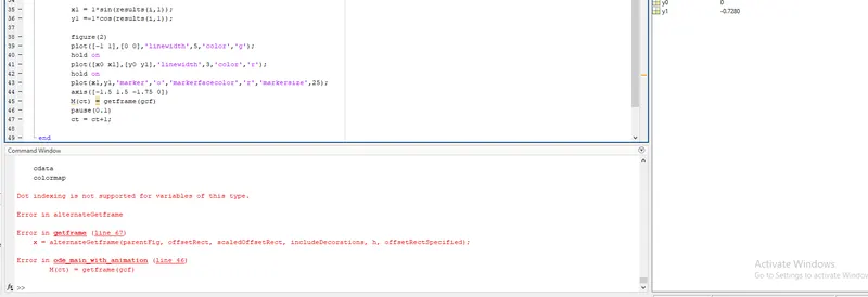
Here the error is about we need to enter the hold off command.The error shown above is corrected by placing the "hold off" function before pause command.

Another error is shown in the movie command that is the m should be in the lowe case letter.

Animation Video of the Motion of the Simple pendulum:

https://youtu.be/VRxAYx5HyeE

Conclusion:

Understand the program to simulate the motion of simple pendulum.