Week 4 - Genetic Algorithm

OPTIMIZATION OF STALAGMITE FUNCTION USING GENETIC ALGORITHM IN MATLAB

AIM:

To study about genetic algorithm and find the global maxima using the genetic algorithm concept to code in MATLAB.

OBJECTIVE:

1. Write a code in MATLAB to optimize the stalagmite function and find the global maxima of the function.
2. Explain the concept of genetic algorithm and explain about the syntax of genetic algorithm.

STALAGMITE FUNCTION:

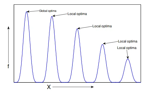
Stalagmite function is a mathematical model that helps to generate maxima’s and minima. Global maxima are a maximum peak value in entire function and global minima is a minimum peak in entire function. But local maxima and local minima are multiple number of values.

Optimization is finding of maxima and minima in particular function but in genetic algorithm its only find minima.

GENETIC ALGORITHM:

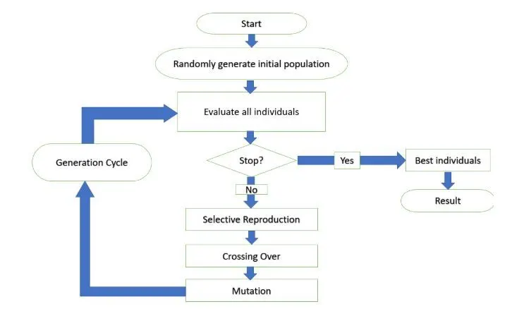
A genetic algorithm is a search heuristic that is inspired by Charles Darwin’s theory of natural evolution. This algorithm reflects the process of natural selection where the fittest individuals are selected for reproduction in order to produce offspring of the next generation. Here the flowchart are given below,

GA OPERATORS AND PARAMETERS:

• Selection
• Crossover
• Mutation

Selection:

The process that determines which solutions are to be preserved and allowed to reproduce and which ones deserve to die out.

The process that determines which solutions are to be preserved and allowed to reproduce and which ones deserve to die out.

The different techniques to implement selection in genetic algorithms,

• Tournament selection
• Roulette wheel selection
• Proportionate selection
• Rank selection
• Steady state selection

Crossover:

The crossover operator is used to create new solutions from the existing solutions available in the mating pool after applying selection operator. This operator exchanges the gene information between the solutions in the mating pool.

Mutation:

Mutation is the occasional introduction of new features in to the solution strings of the population pool to maintain diversity in the population.

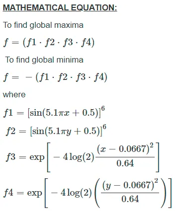
Mathematical model for stalagmite function:

MATLAB CODE:

A function calling program of stalagmite function,

function[f] = stalagamite(input_vector);
x = input_vector(1);
y = input vector(2);
f1_x = sin(5.1*pi*x+0.5)]^6;
f1_y =[sin(5.1*pi*y+0.5)]^6;
f2_x = exp(-4log(2)*)(((x-0.667)^2)/(0.64)));
f2_y = exp(-4*log(2)*(((y-0.667)^2)/(0.64)));

f = (f1_x*f1_y+f2_x*f2_y);
end

A program to optimize the stalagmite function of the global maxima of a function:

clear all 
close all
clc

% Defining our search space
x=linspace(0,0.6,150);
y=linspace(0,0.6,150);

% Creating the 2D mesh
[xx yy] = meshgrid(x,y);

% Evaluating stalagamite fumction
 for i=1:length(xx)
     for j=1:length(yy)
         input_vector(1)=xx(i,j);
         input_vector(2)=yy(i,j);
         f(i,j)=stalagmite(input_vector);
     end
 end
 figure(1)
 surfc(xx,yy,-f)
 xlabel('X VALUE')
 ylabel('Y VALUE')
 
 shading interp
 [inputs,fval] = ga(@stalagmite,2);
 % Study1 statistical behaviour
 num_case = 150;
 tic
 for i=1:num_case
     [inputs,fopt(i)]=ga(@stalagmite,2);
      xopt(i)=inputs(1);
       yopt(i)=inputs(2);
 end
 study_time_1 = toc;
 figure(1)
 subplot(2,1,1)
 hold on
 surfc(x,y,-f)
 shading interp
 plot3(xopt,yopt,-fopt,'marker','o','markersize',5,'markerfacecolor','g')
 title('Únbounded inputs')
 subplot(2,1,2)
 plot(fopt)
 xlabel('iterations')
 ylabel('Function maximum')
 
 % Study2_statical behaviour with upper and lower bounds
 tic
 for i = 1:num_case
     [inputs,fopt(i)]=ga(@stalagmite,2,[],[],[],[],[0:0],[0.7:0.7]);
     xopt(i)=inputs(1);
     ypot(i)=inputs(2);
 end
 study_time_2=toc
 figure(2)
 subplot(2,1,1)
 hold on
 surfc(x,y,-f)
 shading interp
 plot3(xopt,yopt,-fopt,'marker','o','markersize',5,'markerfacecolor','g')
 title('Bounded inputs')
 subplot(2,1,2)
 plot(fopt)
 xlabel('iterations')
 ylabel('Function maximum')
 
 % Study3_Statistical behaviour increasing the ga iterations
 tic
 options=optimoptions('ga');
 options=optimoptions(options,'populationsize',400)
 for i=1:num_case
     [inputs,fopt(i)]=ga(@stalagmite,2,[],[],[],[],[0:0],[0.7:0.7],[],[],options);
     xopt(i)=inputs(1);
     yopt(i)=inputs(2);
 end
 study_time_3=toc
 figure(3)
 subplot(2,1,1)
 hold on 
 surfc(x,y,-f)
 shading interp
 plot3(xopt,yopt,-fopt,'marker','o','markersize',5,'markerfacecolor','g')
 title('Bounded inputs with increased population size')
 subplot(2,1,2)
 plot(fopt)
 xlabel('iterations')
 ylabel('function maximum')
 

CODE EXPLANATION:

1. The program starts with clear all, close all, clc to clear the workspace and old plots.
2. X and y are input 1D arrays, linspace is used to have 150 elements within 0 to 0.6
3. N is the initial population sample size which is one of the critical parameters in genetic algorithms.
4. Mesh grid is used to create 2D arrays with 1D arrays.
5. For loop are used to evaluate the stalagmite function ie:for length of 2D matrix xx&yy.for every value of xx&yy we have defined an input vector(1) &input vector(2),which changes at every iteration performed until the for loop terminates.
6. The values for x&y at function program is taken from these input vectors.
7. f(I,j) is the solution vector which is now an 2D matrix, whose values are calculated by function program.
8. Surfc is used to plot our stalagmite curve in 3D.
9. Shaping interp gives the smooth curve and also eliminates the lines on curves.
10. Ga is now performed syntax as follows

x = ga(fun,nvars) finds a local unconstrained minimum, x, to the objective function, fun. nvars is the dimension (number of design variables) of fun.

11. [inputs,fval] = ga(@stalagmite,2) it refers that fval is the function value at respective inputs,ganis the algorithm solver and stalagmite is our function program call followed by 2 stands for number of variables.

Case 1 :

1. Tic &toc are used to calculate the time taken to perform the simulations.
2. [inputs,fopt(k)]=ga(@stalagmite,2) it refers that fopt(k) is the function value at respective inputs,ga is the algorithm solver & stalagmite is our function program call followed by 2 stands for number of variables.
3. The same as been plotted in a single figure using subplot command.
4. Plot 3 command is used to mark points on 3D space at every intersection of ga calculated xopt, yopt, fopt.
5. Plot(-fopt) is plotted to indicate the maxima values at every iteration.

-f7-fopt are used in the plot command to provide a proper structure and avoid flipping/inverse of plots.

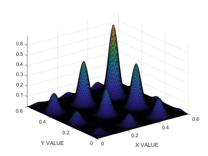
Plot for general Stalagmite model:

Case 1: Unbounded conditions:

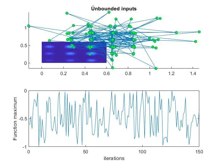
Linspace for both axis x and y from 0 to 0.6 for 150 values.

Giving number cases as 150, genetic algorithm runs up to 150 times and calculate study time for 150 iterations.in this case we calculate the statistical behaviour of stalagmite function by using for loop as ga(@stalagmite) and calculate study time with tic and toc command and then subplot the figure and giving the surfc command to create 3D plot and shading interp command. To plot multiple set co-ordinates we use plot3 command with (x,y,f) and titled as unbounded input commands and to further label the plot we use x label as iteration and y label as function minimum and study time 1 has been calculated.

Case 2: Bounded inputs

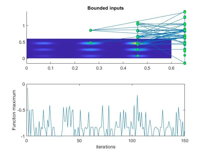
In this case we calculate the statistical behaviour of stalagmite function by setting up lower and upper bounds, where lb(x1,y1) is (0,0) and ub(x2,y2) is (1,1) by this change we can notice that there is decrease in study time. Apart from this same step to be followed as case case 1.

x = ga(fun,nvars,A,b,Aeq,beq,lb,ub) defines a set of lower and upper bounds on the design variables, x, so that a solution is found in the range lb ≤ x ≤ ub. (Set Aeq=[] and beq=[] if no linear equalities exist.)

[inputs,fopt(i)]=ga(@stalagmite,2,[],[],[],[],[0:0],[0.7:0.7]);

Case 3: Bounded inputs with increased population size

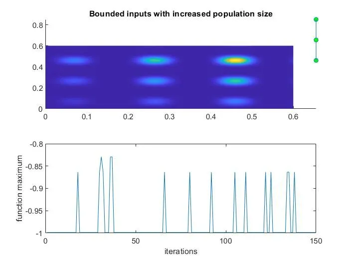
In this case we calculate the statistical behaviour of increasing the ga iterations. Population size has been increased to 400 and ga starts with random variables as there as 2 variables, we will be having 150 sets of 2 rando variables as we increase the population, we get global maxima. Apart from this same step to be followed as case 1 &2.

x = ga(fun,nvars,A,b,Aeq,beq,lb,ub,nonlcon,options) minimizes with the default optimization parameters replaced by values in options. (Set nonlcon=[] if no nonlinear constraints exist.) Create options using optimoptions.

[inputs,fopt(i)]=ga(@stalagmite,2,[],[],[],[],[0:0],[0.7:0.7],[],[],options);

In these above syntax, options refers to our newly defined population size.

Workspace values:

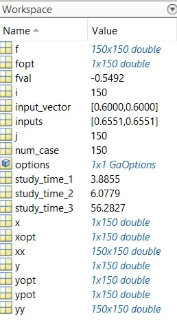
Here the workspace and study time values are plotted.

Conclusion:

When multiple number of iteration runs, GA becomes optimum or linear. The significance of num cases is to check over consistency of output values of ga whether it gives same output for all iterations, so that it can undergoes optimum value.

If we provide less iteration and run the program,ga may or may not able to find global maxima.but,as no.of iteration increases probability of finding global maxima can also increases. When population size increases with iteration probability of global maxima can be optimized.

Thus, the global maxima of the stalagmite function is optimized using genetic algorithm in MATLAB.

References:

1. Microsoft PowerPoint - Genetic Algorithms (iitg.ac.in)
2. OPTIMISATION OF STALAGMITE FUNCTION USING GENETIC ALGORITHM IN MATLAB : Skill-Lync (skill-lync.com)
3. Find minimum of function using genetic algorithm - MATLAB ga - MathWorks India
4. International Journal of Computer Science and Intelligent Computing (IJCSIC) (ijrter.com)
5. Genetic Algorithms.pdf - R.K Bhattacharjya\/CE\/IITG 1 Introduction To Genetic Algorithms Dr Rajib Kumar Bhattacharjya Professor Department of Civil | Course Hero