Project 2 - Rankine cycle Simulator

RANKINE CYCLE SIMULATOR

Aim:

To write a MATLAB code to simulate Rankine cycle.

Objective:

1. Create a Rankine cycle simulator using MATLAB.
2. MATLAB code should calculate the state points of the Rankine cycle based on user inputs.
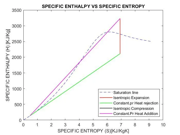
3. Plot the corresponding T-S and H-S plots for the given set of inputs.
4. Calculate the net -work output
5. Back work ratio.

Introduction:

The Rankine cycle is the thermodynamic cycle which converts heat into work. The heat is supplied externally to a closed loop, which usually uses water as the working fluid. This cycle generates about 80% of all electric power used throughout the world, including virtually all solar thermal, biomass, coal and nuclear power plants.

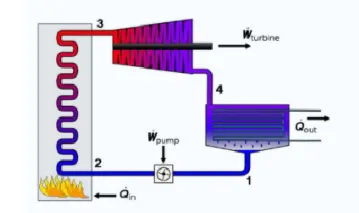
A Rankine cycle describes a model of the operation of steam heat engines most commonly found in power generation plants.

The efficiency of Rankine cycle usually limited by working fluid. The Rankine cycle is sometimes referred to as a practical Carnot cycle. The actual efficiency of 42% for a modern coal-fired power station.

Processes of the Rankine cycle:

T-S diagram of typical Rankine cycle operating between pressures of 0.05 bar and 30 bar.

There are four processes in the Rankine cycle, each changing the state of the working fluid. These states are identified by number in the diagram to the right.

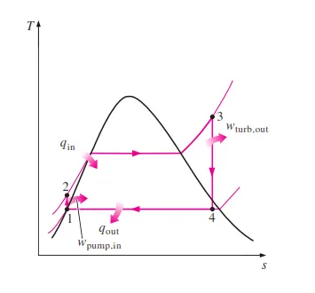
• Process 1-2: The working fluid is pumped from low to high pressure, as the fluid is a liquid at this stage the pump requires little input energy.
• Process 2-3: The high-pressure liquid enters a boiler where it is heated at constant pressure by an external heat source to become a dry saturated vapor.
• Process 3-4: The saturated vapor expands through a turbine, generating power. This decreases the temperature and pressure of the vapor, and some condensation may occur.
• Process 4-1: The wet vapor then enters a condenser where it is condensed at a constant pressure and temperature to become a saturated liquid. The pressure and temperature of the condenser is fixed by temperature of the cooling coils as the fluid is undergoing a phase-change

Governing Equations:

1. Net Work done (W_NET) = W_TURBINE – W_PUMP
2. Thermal Efficiency = W_NET/Q_IN
3. Q_IN = h3-h2
4. Q_OUT = h4-h1
5. W_pump = h2 – h1
6. W_turbine = h3 – h4
7. Back Work Ratio = h1-h4/h2-h3

• Where h1,h2,h3,h4 - the specific enthalpies at indicated points on the T-S diagram.
• Qin – heat supplied to the boiler, Q_out – Output temperature of the boiler.
• W_pump,W_turbine - Work done by turbine and pump.

Required Inputs:

1. Turbine inlet temperature – 400 degree Celsius.
2. Turbine inlet pressure – 30 bar
3. Turbine outlet pressure – 0.05 bars = condenser Inlet pressure.

MATLAB code for Rankine Cycle Simulator:

clear all
close all
clc


   fprintf('\n')
   disp(' RANKINE CYCLE SIMULATOR')
   disp('Process 1-2:Isentropic expansion in turbine')
   disp('Process 2-3:Constant pressure heat rejection in condensor')
   disp('Process 3-4:Isentropic compression in pump')
   disp('process 4-1:Constant pressure heat addition in boiler')

   % User inputs
   %p1=30;
   %p2=0.05;
   %t1=400;
   fprintf('\n')
   p1 =30;
   t1=400;
   p2=0.05;
   
   % Extracting data from XSteam
   
  s2_f = XSteam('sL_p',p2);
  s2_g = XSteam('sV_p',p2);
  s2_fg = s2_g-s2_f;
  t1_sat = XSteam('Tsat_p',p1);
  t2_sat = XSteam('Tsat_p',p2);
  cp2_g = XSteam('CpV_p',p2);
  h2_f = XSteam('hL_p',p2);
  h2_g = XSteam('hV_p',p2);
  h2_fg = h2_g - h2_f;
  s4_f = XSteam('sL_p',p1);
  cp4_f = XSteam('CpL_p',p1);
  s1_ = XSteam('sV_p',p1);
  s2_ = XSteam('sV_p',p2);
  s4_ = XSteam('sL_p',p1);
  v3=XSteam('vL_p',p2);
 
  
  % Process 1-2: isentropic expansion of steam
  if t1>t1_sat
      h1 = XSteam('h_pT',p1,t1);
      s1 = XSteam('s_pT',p1,t1);
  else
      h1 = XSteam('hV_p',p1);
      s1 = XSteam('sV_p',p1);
  end
  
  s2 = s1;
  x2 = (s2-s2_f)/s2_fg;
  
  if x2>1
      t2 = t2_sat*exp((s2 - s2_g)/cp2_g);
      h2 = XSteam('h_pT',p2,t2);
  else
      t2 = t2_sat;
      h2 = h2_f + (x2 * h2_fg);
  end
  % Process 2-3:Constant pressure heat rejection
  h3 = h2_f;
  s3 = s2_f;
  t3 = t2_sat;
  p3 = p2;
  
  % Process 3-4: Isentropic compression in pump
  
  p4 = p1;
  pump_work = v3*(p1-p2)*100;
  h4 = pump_work + h3;
  s4 = s3;
  t4 = t1_sat/ exp((s4_f-s4)/cp4_f);
  
  % Turbine work 
  Turbine_work = (h1-h2);
  
  % Heat supplied by boiler 
  
  Heat_supplied = (h1-h4);
  
  % Shaft work
  
  Shaft_work = (Turbine_work - pump_work);
  
  % Efficiency of rankine cycle
  
  n_rankine = (Shaft_work/Heat_supplied)*100;
  
  % Back work ratio
  
  Back_work = (pump_work/Turbine_work);
  
  % Display the results
  
  fprintf('\n')
  disp('Parameters at State Point-1')
  fprintf('P1 : %.2f BAR\n',p1)
  fprintf('T1 : %.2f °C\n',t1)
  fprintf('H1 : %.2f KJ/Kg\n',h1)
  fprintf('S1 : %.2f KJ/KgK\n',s1)
  
  fprintf('\n')
  disp('Parameters at state point-2')
  fprintf('P2 : %.2f BAR\n',p2)
  fprintf('T2 : %.2f °C\n',t2)
  fprintf('H2 : %.2f KJ/Kg\n',h2)
  fprintf('S2 : %.2f KJ/KgK\n',s2)
  fprintf('X2 : %.2f\n',x2)
  
  fprintf('\n')
  disp('Parameters at state point-3')
  fprintf('P3 : %.2f BAR\n',p3)
  fprintf('T3 : %.2f °C\n',t3)
  fprintf('H3 : %.2f KJ/Kg\n',h3)
  fprintf('S3 : %.2f KJ/KgK\n',s3)
  
   fprintf('\n')
  disp('Parameters at state point-4')
  fprintf('P4 : %.2f BAR\n',p4)
  fprintf('T4 : %.2f °C\n',t4)
  fprintf('H4 : %.2f KJ/Kg\n',h4)
  fprintf('S4 : %.2f KJ/KgK\n',s4)
  
  fprintf('\n')
  fprintf('Pump Work        :%.2f KJ/kg\n',pump_work)
  fprintf('Turbine Work     :%.2f KJ/kg\n',Turbine_work)
  fprintf('Shaft Work       :%.2f KJ/kg\n',Shaft_work)
  fprintf('Thermal Efficiency :%.2f PERCENT\n',n_rankine)
  fprintf('\n Backwork Ratio:%.5f\n',Back_work)
  
  % Plotting liquid /vapour lines
  
  t = linspace(0,400,200);
  for i =1:length(t)
      hl(i) = XSteam('hL_T',t(i));
      hv(i) = XSteam('hV_T',t(i));
      sl(i) = XSteam('sL_T',t(i));
      sv(i) = XSteam('sV_T',t(i));
      
  end
  
  figure(1)
  
  plot([sl,sv],[t,t],'--','color','b')
  hold on
  plot([s3,s4,s4_],[t3,t4,t1_sat],'linewidth',1,'color','r')
  hold on
  plot([s4_,s1_,s1],[t1_sat,t1_sat,t1],'linewidth',1,'color','g')
  hold on
  plot([s1,s2],[t1,t2],'linewidth',1,'color','m')
  hold on
  
  if x2>1
      plot([s2,s2_,s3],[t2,t2_sat,t2],'linewidth',1,'color','y')
  else
      plot([s2,s3],[t2,t3],'linewidth',1,'color','m')
  end
  axis ([0 18 -5 (t1+200)])
  xlabel('SPECIFIC ENTROPY (S) [KJ/KgK]')
  ylabel('TEMPERATURE (T) [°C]')
  title('TEMPERATURE vs SPECIFIC ENTROPY')
  legend('Saturation Line','Isentropic Compression in Pump','Constant Pressure Heat Addition','Isentropic Expansion in Turbine','Constant Pressure Heat rejection in Condenser')
  
  % Plotting H-S Diagram
  figure(2)
  plot([sl,sv],[hl,hv],'--','color','b')
  hold on
  plot([s1,s2],[h1,h2],'linewidth',1,'color','r')
  hold on
  plot([s2,s3],[h2,h3],'linewidth',1,'color','g')
  hold on
  plot([s3,s4],[h3,h4],'linewidth',1,'color','k')
  hold on
  plot([s4,s1],[h4,h1],'linewidth',1,'color','m')
  xlabel('SPECIFIC ENTROPY (S)[KJ/KgK]')
  ylabel('SPECIFIC ENTHALPY (H) [KJ/Kg]')
  title('SPECIFIC ENTHALPY VS SPECIFIC ENTROPY')
  legend('Saturation line','Isentropic Expansion','Constant.pr Heat rejection','Isentropic Compression','Constant.Pr Heat Addition','location','southeast')

Output Screen:

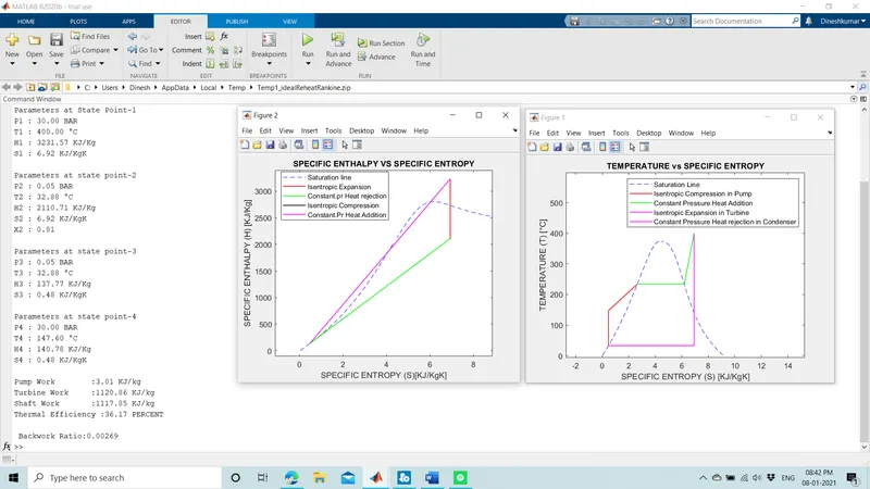
PLOTS:

1. Temperature vs Specific Entropy

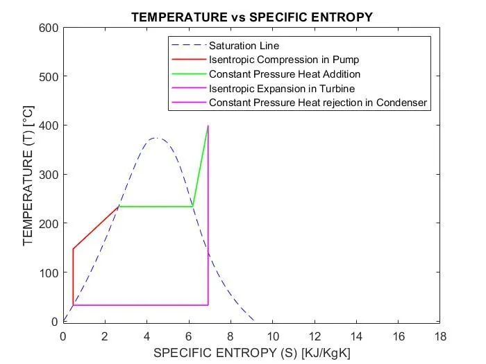
2.Specific Entropy vs Specific Enthalpy

Conclusion:

Thus, the given inputs, output was obtained by using the XSTEAM table and Rankine cycle simulation was done.

References:

1. (PDF) Rankine cycle | Ravindra Patil - Academia.edu
2. Ch9, Lesson B, Page 7 - Efficiency & Back Work Ratio (learnthermo.com)
3. Rankine Cycle Simulator : Skill-Lync (skill-lync.com)