Week 3 - Solving second order ODEs

AIM:

Write a MATLAB program to solve the second order ode with help of simple pendulum.

GOVERNING EQUATIONS:

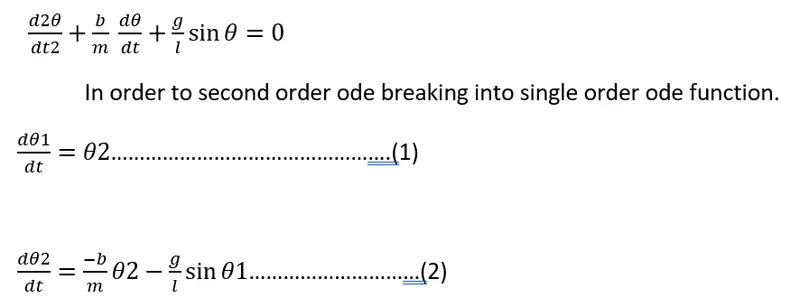
This equation can be solved ode45 solver to already build in the MATLAB function.

CODE EXPLANATION:

1. Given input variables are,

b=0.05 for damping coefficient

l=1 m for length of the pendulum

m=1 kg for mass

g=9.81 m/s2 for gravity act on the pendulum

Motion between 0-20sec given and Angular displacement=0 and angular velocity=3rad/sec with respect to the time t = 0.

2. Initial condition angular velocity 0 and angular displacement 5 are initializing.
3. Time points are defined 0 to 10 splits into 500 values using the command linspace.
4. Ode45 solver is already build in MATLAB functions, that function provide dependant and independent variables along with the functions, integration limit and initial conditions are provided. Calling a function to be separated to the other workspace.
5. Plotting the angular displacement and angular velocity in various time points.
6. Set the counter value ct=1, and initialize the for loop for execute the loop for no of times for starting value and ending value should be given.
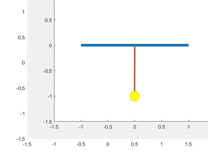
7. Plotting the animation
8. Animation of pendulum for to create the movie file and video file & video writer with respect to the corresponding MATLAB coding file with completing .avi pattern
9. Open a video file and write video for file and movie after, that closing the video file.

MAIN PROGRAM:

clear all
close all
clc
%Inputs for simple pendulum
b=0.05;
g=9.81;
l=1;
m=0.1;
%Initial Condition
theta_0=[0;3];
%Time points
t_span=linspace(0,20,500);
%Solve ode
[t,results]=ode45(@(t,theta) odefunction(t,theta,b,g,l,m),t_span,theta_0);
% Plotting
plot(t,results(:,1))
hold on 
plot(t,results(:,2))
title('DAMPED HARMONIC MOTION OF PENDULUM')
legend('ANGULAR DISPLACEMENT','ANGULAR VELOCITY')
xlabel('TIME')
ylabel('POSITION-PLOT')

%Initializing the for loop

ct=1;
for i=1:length(results(:,1))
    x_start=0
    y_start=0
    x_end=l*sin(results(i,1))
    y_end=-l*cos(results(i,1))
    
    % plotting the animation
    figure(2)
    plot([-1 1],[0 0], 'linewidth',5)
    hold on 
    plot([x_start x_end ],[y_start y_end],'linewidth',3)
    hold on 
    plot(x_end,y_end,'o','markersize',20,'markerfacecolor','y')
    title('ANIMATION OF TRANSIENT BEHAVIOUR OF PENDULUM')
    axis([-1.5 1.5 -1.5 1])
    pause(0.03)
    hold off
    
    
   M(ct)=getframe(gcf)
    ct=ct+1;
end

% Animation of pendulum

movie(M)
videofile = VideoWriter('secondorderode.avi','uncompressed avi')
open(videofile)
writeVideo(videofile,M)
close(videofile)

FUNCTION PROGRAM:

function [dtheta_dt] = odefunction(t,theta,b,g,l,m)
theta1 = theta(1);
theta2 = theta(2);
dtheta1_dt =theta(2);
dtheta2_dt = -(b/m)*theta2-(g/l)*sin(theta1);
dtheta_dt = [dtheta1_dt ; dtheta2_dt]
end

PLOTS:

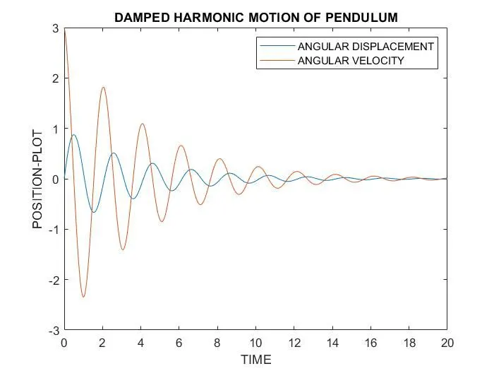
Plot for angular displacement and angular velocity with respect to the time.

VIDEO LINK: https://youtu.be/Qsmq22n5GYs

RESULTS:

After that calculating the results, a graph has been plotted, the graph contains two plots angular displacement with respect to time and angular velocity with respect to time. Hence the transient behaviour of simple pendulum was successfully created by using the MATLAB functions.