Genetic Algorithm

Aim:

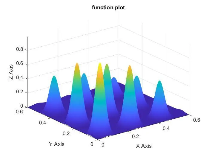
To write a program code to optimise the stalagmite function and find the global maxima of the function.

Genetic Algorithm:

Genetic Algorithm (GA) is a search-based optimization technique based on the principles of Genetics and Natural Selection. It is frequently used to find optimal or near-optimal solutions to difficult problems which otherwise would take a lifetime to solve. It is frequently used to solve optimization problems, in research, and in machine learning.

The genetic algorithm is a method for solving both constrained and unconstrained optimization problems that is based on natural selection, the process that drives biological evolution. It repeatedly modifies a population of individual solutions. At each step, the genetic algorithm selects individuals at random from the current population to be parents and uses them to produce the children for the next generation. Over successive generations, the population "evolves" toward an optimal solution. You can apply the genetic algorithm to solve a variety of optimization problems that are not well suited for standard optimization algorithms, including problems in which the objective function is discontinuous, nondifferentiable, stochastic, or highly nonlinear. The genetic algorithm can address problems of mixed integer programming, where some components are restricted to be integer-valued.

Genetic Algorithm in matlab is a solver "ga" and the syntax used is as follows

ga(fun,nvars,A,b,[],[],lb,ub,nonlcon,IntCon,options)

where,

fun — Objective function

nvars — Number of variables

A — Linear inequality constraints

b — Linear inequality constraints

Aeq — Linear equality constraints

beq — Linear equality constraints

lb — Lower bounds

ub — Upper bounds

nonlcon — Nonlinear constraints

IntCon — Integer variables

options — Optimization options

Stopping Conditions for the Algorithm:

The genetic algorithm uses the following options to determine when to stop. See the default values for each option by running opts = optimoptions('ga').

MaxGenerations — The algorithm stops when the number of generations reaches MaxGenerations.

MaxTime — The algorithm stops after running for an amount of time in seconds equal to MaxTime.

FitnessLimit — The algorithm stops when the value of the fitness function for the best point in the current population is less than or equal to FitnessLimit.

MaxStallGenerations — The algorithm stops when the average relative change in the fitness function value over MaxStallGenerations is less than Function tolerance.

MaxStallTime — The algorithm stops if there is no improvement in the objective function during an interval of time in seconds equal to MaxStallTime.

FunctionTolerance — The algorithm runs until the average relative change in the fitness function value over MaxStallGenerations is less than Function tolerance.

ConstraintTolerance — The ConstraintTolerance is not used as stopping criterion. It is used to determine the feasibility with respect to nonlinear constraints. Also, max(sqrt(eps),ConstraintTolerance) determines feasibility with respect to linear constraints.

The algorithm stops as soon as any one of these conditions is met.

Optimization of 'ga':

optimization depends on the following,

i. Selection: Selection of individuals happens as per the fitness level.

ii. Cross Over: Convergence towards local maxima/minima.

iii. Mutation: process of finding the better maxima/minima.

Governing equation for stalagmite function:

f_1,x = [sin(5.1 . π . x + 0.5)]⁶

f_1,y = [sin(5.1 . π . y + 0.5)]⁶

f_2,x = `exp(-4 . l o g (2). (x - 0.0667)^2/0.64)`

f_2,x = `exp(-4 . l o g (2). (y - 0.0667)^2/0.64)`

Program:

Stalagmite Function:

function[F] = stalagmite(input_vector)
x1 = input_vector(1);
y1 = input_vector(2);
f1_x = (sin(5.1 * pi * x1 +0.5)).^6;
f1_y = (sin(5.1 * pi * y1 +0.5)).^6;
f2_x = exp(-4 * log(2) * ((x1 - 0.0667).^2)/0.64);
f2_y = exp(-4 * log(2) * ((y1 - 0.0667).^2)/0.64);
F = -(f1_x .* f2_x .* f1_y .* f2_y);
end

Main Program:

% Program to optimise the stalagmite function and find the global maxima

% Defining search space
x = linspace(0,0.6, 150);
y = linspace(0,0.6, 150);

% 2D Mesh
[xx yy] = meshgrid(x,y);

% Evaluating stalagmite function
for i = 1:length(xx)
    for j = 1:length(yy)
        input_vector(1) = xx(i,j);
        input_vector(2) = yy(i,j);
        f(i,j) = stalagmite(input_vector);
    end
end

figure(1)
surfc(xx,yy,-f)
shading interp
xlabel('X Axis')
ylabel('Y Axis')
zlabel('Z Axis')
title('function plot')

% No of iterations
cases = 50;

% Study 1 : Statistical behaviour

tic
for i = 1:cases
    [inputs, fval(i)] = ga(@stalagmite, 2);
    xout(i) = inputs(1);
    yout(i) = inputs(2);
end

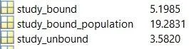
study_unbound = toc

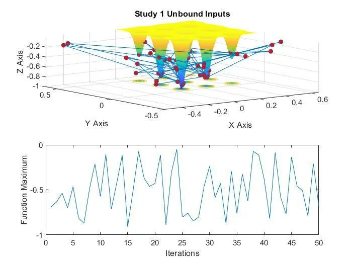
figure(2)
subplot(2,1,1)
surfc(xx, yy, f)
shading interp
hold on
plot3(xout, yout, fval, 'marker', 'o', 'markersize', 5, 'markerfacecolor', 'r')
xlabel('X Axis')
ylabel('Y Axis')
zlabel('Z Axis')
title('Study 1 Unbound Inputs')
subplot(2,1,2)
plot(fval)
xlabel('Iterations')
ylabel('Function Maximum')

% Study 2 statistical Behaviour with Bounded Inputs

tic
for i = 1:cases
    [inputs1, fval1(i)] = ga(@stalagmite, 2,[],[],[],[],[0;0],[0.5;0.5]);
    xout1(i) = inputs1(1);
    yout1(i) = inputs1(2);
end

study_bound = toc

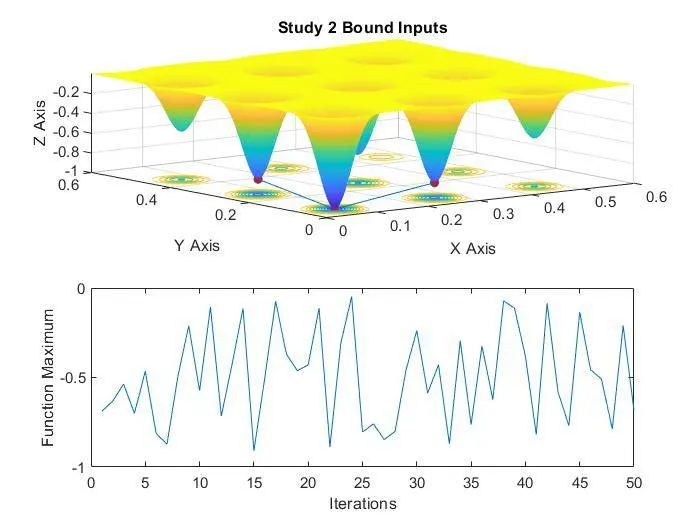
figure(3)
subplot(2,1,1)
surfc(xx, yy, f)
shading interp
hold on
plot3(xout1, yout1, fval1, 'marker', 'o', 'markersize', 5, 'markerfacecolor', 'r')
xlabel('X Axis')
ylabel('Y Axis')
zlabel('Z Axis')
title('Study 2 Bound Inputs')
subplot(2,1,2)
plot(fval)
xlabel('Iterations')
ylabel('Function Maximum')

% Case 3 Bounded with fixed population

tic

options = optimoptions('ga','populationSize', 250)

for i = 1:cases
    [inputs2, fval2(i)] = ga(@stalagmite, 2,[],[],[],[],[0;0],[0.5;0.5],[],options);
    xout2(i) = inputs2(1);
    yout2(i) = inputs2(2);
end
study_bound_population = toc

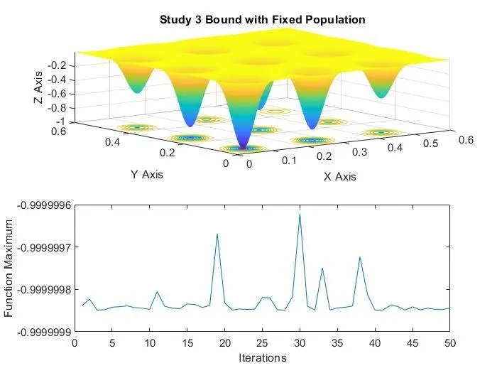
figure(4)
subplot(2,1,1)
surfc(xx, yy, f)
shading interp
hold on
plot3(xout2, yout2, fval2, 'marker', 'o', 'markersize', 5, 'markerfacecolor', 'r')
xlabel('X Axis')
ylabel('Y Axis')
zlabel('Z Axis')
title('Study 3 Bound with Fixed Population')
subplot(2,1,2)
plot(fval2)
xlabel('Iterations')
ylabel('Function Maximum')

Explanation:

• Lines 4 to 8 inputs to generate a matrix values.
• Lines 10 to 17 for each value generated the program runs the stalagmite function and generates an output.
• Lines 19 to 25 plots the graph as shown in figure 1.
• Line 28 defines the number of iterations input.
• Lines 33 to 37 generates output with the help of ga command defined.
• tic and toc is used to generate the time taken by the program.
• Lines 41 to 54 plots the graph as shown in figure 2.
• Lines 59 to 63 generates output with the help of ga command defined i.e. with boundry conditions set.
• Lines 67 to 80 plots the graph as shown in figure 3.
• Line 86 input parameter option is defined i.e. population size is defined.
• Lines 88 to 92 generates output with the help of ga command defined i.e. with boundry and population set.
• Lines 95 to 108 plots the graph as shown in figure 4.

Output:

Time Study:

Reference:

mathworks.com/help/gads/ga.html