Genetic Algorithm
AIM:- To write a code in MATLAB to optimise the Stalagmite function and find the global maxima of the function.
THEORY:-
(1) About GA:-
It is based upon evolution theory.
In Operation research, Genetic Algorithm is defined as the process of natural selection that belongs to larger class of evolutionary algorithms.
A Genetic Algorithm is a metod for solving both constrained and unconstrained optimization problems based on a natural selection process that mimics biological evolution. The algorithm repeatedly modifies a population of individual solutions.
At each step genetic algorithm randomly selects individuals from the current population and uses them as parents to produce the children for next generation.
Genetic Algorithm are commomnly used to generate high quality solutions to optimisation and search problems by relying on biological factors.
(2) OPTIMISATION:-
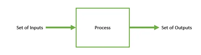
An area of study that deals with how to minimize or maximize a particular function which depend on multiple input parameters. Optimization refers to finding the values of inputs in such a way that we get the best output values. The definition of best depends on problem to problem but in mathematical terms it refers to maximizing or minimizing one or more objective function.
The set of all possible solutions or values which the inputs can take up the search space. The aim of optimization is to find that point or set of points in search space.
There are several methods to go about optimisation:-
The one of the method is Stalagmite Function.
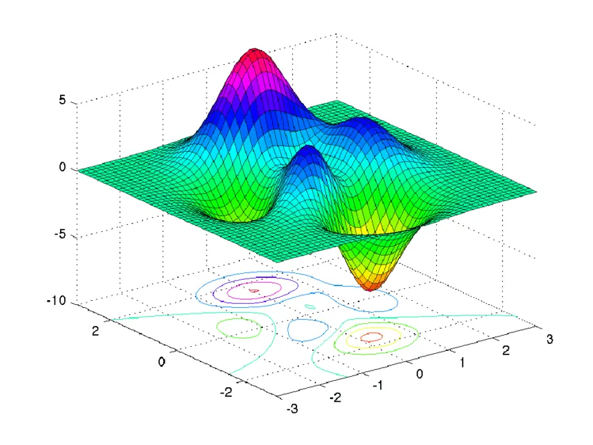
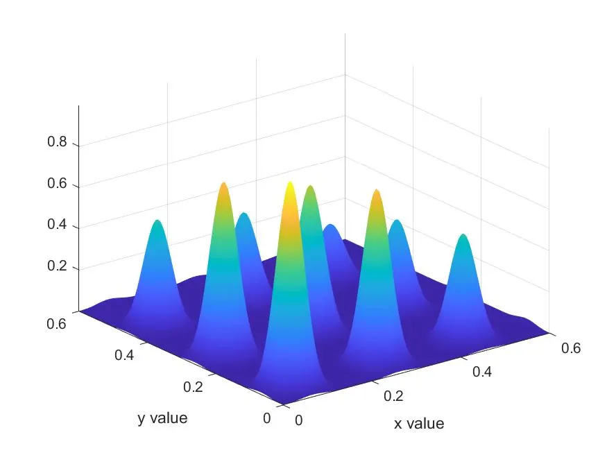
(3) Stalagmite Function is the mathematical model that actually helps us generate local minima and maxima.
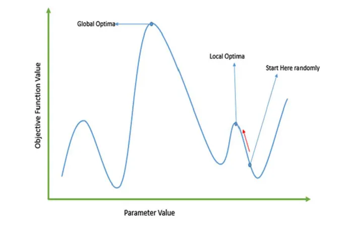
Local maxima = Tiny peaks.
Global maxima = huge peaks = point at corner.
(4) STOPPING CRITERIA:-
The termination condition of a GA is important in determining when GA run will end. It has been observed that initially, the GA progress very fast with better solutions coming in every few iterations but this tend to saturate in the later stages where the improvements are very small. We usually want a termination condition such that our solution is close to the optimal, at the end of run.
Usually we keep one of the folloing termination conditions:-
1) When there has been no improvement in the population for X-number of generations.
2) When we reach an absolute number of generation.
3) When the objective function has reached a certain predefined value.
SYNTAX FOR GA:-
The syntax used for Genetic Algorithm is {x = ga(fun, nvars), finds a local unconstrained minimum where
x = is the objective function.
nvars = is the dimension (design of variables) of fun.
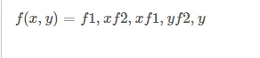
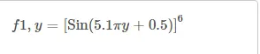
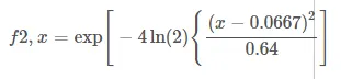
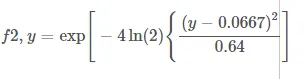
FORMULA USED:- This is the Stalagmite Function formula which is used in the function program.

CODE:-
FUNCTION CODE:- This is the Function code written to run the stalagmite function program.
function [f] = stalagmite(input_vector)

x = input_vector(1);
y = input_vector(2);
f1 = (sin(5.1*pi*x+0.5))^6;
f2 = (sin(5.1*pi*y+0.5))^6;
f3 = exp(-4*log(2)*(x-0.0667)^2/0.64);
f4 = exp(-4*log(2)*(y-0.0667)^2/0.64);

[f] = (f1*f2*f3*f4);
end
PROGRAM CODE:-
This is the basic program to understand the importance of stalagmite function and how these peaks takes place and what are the values of them that is provided in the program.
clear all
close all
clc

% Defining our search space
x = linspace(0,0.6,150);
y = linspace(0,0.6,150);

% Creating a 2Dimensional mesh
[xx,yy] = meshgrid(x,y);

%Evaluating the stalagmite function
for i = 1:length(xx)
    for j = 1:length(yy)
        input_vector(1) = xx(i,j);
        input_vector(2) = yy(i,j);
        f(i,j) = stalagmite(input_vector);
    end
end

surfc(xx,yy,f)
xlabel('x value')
ylabel('y value')
shading interp
[inputs,fval] = ga(@stalagmite,2)
PROCEDURE:-
Step 1:- First write the basic commands whichever needed to start the program.
Step 2:- Now mark the comments by this (%).
Step 3:- Make use of linspace command which is used to find accurate number of values required between the given desired values.
Step 4:- Now i have created a 2Dimension mesh using meshgrid command.
Step 5:- After this use of for loop command which is used to define a number of iterations that is taking place. we put all the values as mentioned above through comments and we apply to it. At last we end the program by providing end commmand.
Step 6:- surfc(xx,yy, f):- it will always gives you the value of minima that is why to calculate z-axis for the reference we have taken f as a reference.
x and y are axis that is taken.
Step 7:- shading interp:- this code is used in matlab to perform shading instead of lines.
tic:- this is used in matlab program and that too above the start of program as it start stopwatch timer.
toc:- this is the code used in the matlab program to start stopwatch timer.
RESULT:-
FUNCTION CODE:- This is the Function code written to run the getstalagmite function program.
function [f] = getstalagmite(inputs)
x = inputs(1);
y = inputs(2);
f1 = (sin(5.1*pi*x+0.5))^6;
f2 = (sin(5.1*pi*y+0.5))^6;
f3 = exp(-4*log(2)*(x-0.0667)^2/0.64);
f4 = exp(-4*log(2)*(y-0.0667)^2/0.64);

[f] = -(f1*f2*f3*f4);
end
PROCEDURE:-
Step1:- In this we have written the For loop code to put all the formulas into it which is going to be used as the formulae used in GA.
Step2:- We have taken a many functions to simulate the formula and placed each and everyone under main function itself.
Step3:- The inputs of x and y are provided into it.
Step4:- Now we save the file and folder name same so that it wont face any problem while running the code.
PROGRAM FOR 3 DIFFERENT CASES:-
clear all
close all
clc

x = linspace(0,0.6,150);
y = linspace(0,0.6,150);
num_cases = 50;

% Creating a 2D mesh
[xx,yy] = meshgrid(x,y);

for i = 1:length(xx)
    for j = 1:length(yy)
    inputs(1)=xx(i,j);
    inputs(2)=yy(i,j);
    f(i,j) = getstalagmite(inputs);
    end
end

tic
 % Study 1 - Statistical behaviour
 for k = 1:num_cases
     [inputs, fopt(k)] = ga(@getstalagmite,2);
     xopt(k) = inputs(1);
     yopt(k) = inputs(2);
 end
 figure(1)
 subplot(2,1,1)
surfc(xx, yy, -f)
 hold on

 shading interp
 plot3(xopt,yopt,-fopt,'marker','o','markersize',5,'markerfacecolor','r')
 title('Unbounded inputs')
 subplot(2,1,2)
 plot(-fopt)
 xlabel('Iterations')
 ylabel('Function minimum')
 study1_time = toc;

 tic
% Study 2 - Statistical behaviour - with upper and lower bounds
 for i = 1:num_cases
     [inputs, fopt(i)] = ga(@getstalagmite,2,[],[],[],[],[0,0],[0.3,0.3]);
     xopt(i) = inputs(1);
     yopt(i) = inputs(2);
end

 figure(2)
 subplot(2,1,1)
 hold on
 surfc(xx, yy, -f)
 shading interp
 plot3(xopt, yopt, -fopt,'marker','o','markersize',5,'markerfacecolor','r')
 title('Bounded inputs')
 subplot(2,1,2)
 plot(-fopt)
 xlabel('Iterations')
 ylabel('Function minimum')
 study2_time = toc;

 tic

% Study 3 increasing GA iteration
options = optimoptions('ga');
options = optimoptions(options,'PopulationSize',150);


for i = 1:num_cases
    [inputs, fopt(i)] = ga(@getstalagmite,2,[],[],[],[],[0,0],[0.3,0.3],[],[],options);
    xopt(i) = inputs(1);
    yopt(i) = inputs(2);
end

figure(3)
subplot(2,1,1)
hold on
surfc(xx, yy, -f)
shading interp
plot3(xopt, yopt, -fopt,'marker','o','markersize',5,'markerfacecolor','r')
title('Bounded inputs')
subplot(2,1,2)
plot(-fopt)
xlabel('Iterations')
ylabel('Function minimum')
study3_time = toc;
Syntax used in the above program:-
(1) surfc(xx,yy,-f):- here (-f) is taken to calculate the maxima because it will always gives you the value of minima that is why to calculate z-axis for the reference we have taken f and that too in negative sign.
x and y are axis that is taken.
(2) shading interp:- this code is used in matlab to perform shading instead of lines.
(3) tic:- this is used in matlab program and that too above the start of program as it start stopwatch timer.
(4) toc:- this is the code used in the matlab program to start stopwatch timer.
STUDY 1:- This program is made for the Statistical Behaviour:-
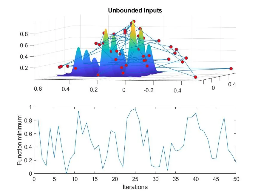
In this program the graph is obtained which has many maxima points and its not specified . For GA program we have given {[inputs, fopt(k)] = ga(@getstalagmite,2)}, which means that the value 2 provided to it is for the 2 maxima points.
clear all
close all
clc

x = linspace(0,0.6,150);
y = linspace(0,0.6,150);
num_cases = 50;

% Creating a 2D mesh
[xx,yy] = meshgrid(x,y);

for i = 1:length(xx)
    for j = 1:length(yy)
    inputs(1)=xx(i,j);
    inputs(2)=yy(i,j);
    f(i,j) = getstalagmite(inputs);
    end
end

tic
 % Study 1 - Statistical behaviour
 for k = 1:num_cases
     [inputs, fopt(k)] = ga(@getstalagmite,2);
     xopt(k) = inputs(1);
     yopt(k) = inputs(2);
 end
 figure(1)
 subplot(2,1,1)
surfc(xx, yy, -f)
 hold on

 shading interp
 plot3(xopt,yopt,-fopt,'marker','o','markersize',5,'markerfacecolor','r')
 title('Unbounded inputs')
 subplot(2,1,2)
 plot(-fopt)
 xlabel('Iterations')
 ylabel('Function minimum')
 study1_time = toc;
PROCEDURE:-
Step 1:- First write all the basic commands.
Step 2:- We have given the values for x and y by using linspace command which is used in the code to give accurate numbers or values whatever asked.
Step 3:- We have provided the num_case command as per the numbers to be used in it.
Step 4:- Now i have used the meshgrid command for the x and y. meshgrid transform the domain specified by vectors x and y into arrays X and Y, which can be used to evaluate functions of two variables and three dimensional mesh surface plots.
Step 5:- Now we have taken the for loop command ang putted the input values as mentioned before, i have given getstalagmite function too in it
Step 6:- surfc(xx,yy,-f):- here (-f) is taken to calculate the maxima because it will always gives you the value of minima that is why to calculate z-axis for the reference we have taken f and that too in negative sign.
x and y are axis that is taken.
Step 7:- shading interp:- this code is used in matlab to perform shading instead of lines.
Step 8:- tic:- this is used in matlab program and that too above the start of program as it start stopwatch timer.
toc:- this is the code used in the matlab program to start stopwatch timer.
Step 9:- Now i have labelled the graphs by x-axis and y-axis.
Step 10:- The title has been given to it for the particular graph
RESULT:-
In this the iteration takes place for 50 times as the input given is num_cases = 50. There is random search so results vary each time. Here some new commands are used into it.
shading interp is used to shade the plot instead of lines.
surfc command is used to create 3Dimensional plot to result space.
Optimisation results were plotted and the negative sign is used to invert the graph to find the maxima points.
We aren't able to receive proper result as everytime the result is changed.
STUDY (2) STATISTICAL BEHAVIOUR:- UPPER AND LOWER BOUNDS.
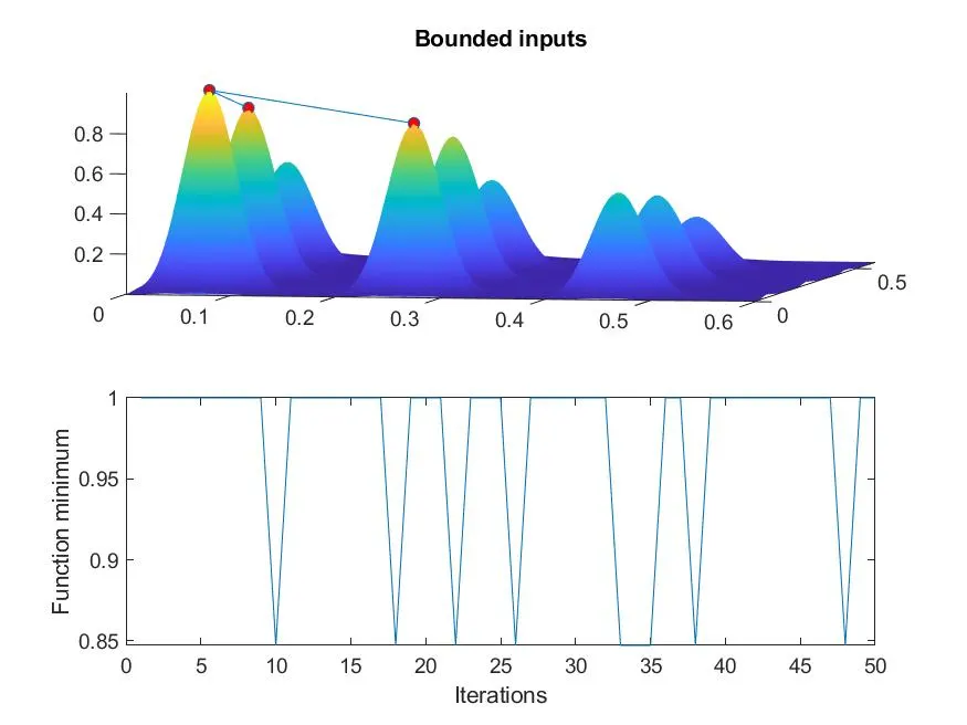
In this program the graph is obtained which has three maxima points. For GA program we have given {[inputs, fopt(i)] = ga(@getstalagmite,2,[],[],[],[],[0,0],[0.3,0.3])}, which means that value of lower bound is 0 and the value of upper bound is 0.3.
Through this we can easily find the values of maxima.
CODE:-
clear all
close all
clc

x = linspace(0,0.6,150);
y = linspace(0,0.6,150);
num_cases = 50;

% Creating a 2D mesh
[xx,yy] = meshgrid(x,y);

for i = 1:length(xx)
    for j = 1:length(yy)
    inputs(1)=xx(i,j);
    inputs(2)=yy(i,j);
    f(i,j) = getstalagmite(inputs);
    end
end

tic
% Study 2 - Statistical behaviour - with upper and lower bounds
 for i = 1:num_cases
     [inputs, fopt(i)] = ga(@getstalagmite,2,[],[],[],[],[0,0],[0.3,0.3]);
     xopt(i) = inputs(1);
     yopt(i) = inputs(2);
end

 figure(2)
 subplot(2,1,1)
 hold on
 surfc(xx, yy, -f)
 shading interp
 plot3(xopt, yopt, -fopt,'marker','o','markersize',5,'markerfacecolor','r')
 title('Bounded inputs')
 subplot(2,1,2)
 plot(-fopt)
 xlabel('Iterations')
 ylabel('Function minimum')
 study2_time = toc;
PROCEDURE:-
Step 1:- First write all the basic commands.
Step 2:- We have given the values for x and y by using linspace command which is used in the code to give accurate numbers or values whatever asked. as we have to find exact values from 0 to 0.6 and a total of exact 150 numbers.
Step 3:- We have provided the num_case command as per the numbers to be used in it.
Step 4:- Now i have used the meshgrid command for the x and y. meshgrid transform the domain specified by vectors x and y into arrays X and Y, which can be used to evaluate functions of two variables and three dimensional mesh surface plots.
Step 5:- Now we have taken the for loop command ang putted the input values as mentioned before, i have given getstalagmite function too in it
Step 6:- surfc(xx,yy,-f):- here (-f) is taken to calculate the maxima because it will always gives you the value of minima that is why to calculate z-axis for the reference we have taken f and that too in negative sign.
x and y are axis that is taken.
Step 7:- shading interp:- this code is used in matlab to perform shading instead of lines.
Step 8:- tic:- this is used in matlab program and that too above the start of program as it start stopwatch timer.
toc:- this is the code used in the matlab program to start stopwatch timer.
Step 9:- Now i have labelled the graphs by x-axis and y-axis.
Step 10:- The title has been given to it for the particular graph
RESULT:-
Here we have found the lower and upper bounds for the search space.
Remaining process is same.
The results are improved but still problem occurs with the maxima points. So as for this we went to 3rd method to find accurate results.
STUDY (3) INCREASING GENETIC ALGORITHM ITERATION:-
CODE:-
clear all
close all
clc

x = linspace(0,0.6,150);
y = linspace(0,0.6,150);
num_cases = 50;

% Creating a 2D mesh
[xx,yy] = meshgrid(x,y);

for i = 1:length(xx)
    for j = 1:length(yy)
    inputs(1)=xx(i,j);
    inputs(2)=yy(i,j);
    f(i,j) = getstalagmite(inputs);
    end
end

tic
% Study 3 increasing GA iteration
options = optimoptions('ga');
options = optimoptions(options,'PopulationSize',150);


for i = 1:num_cases
    [inputs, fopt(i)] = ga(@getstalagmite,2,[],[],[],[],[0,0],[0.3,0.3],[],[],options);
    xopt(i) = inputs(1);
    yopt(i) = inputs(2);
end

figure(3)
subplot(2,1,1)
hold on
surfc(xx, yy, -f)
shading interp
plot3(xopt, yopt, -fopt,'marker','o','markersize',5,'markerfacecolor','r')
title('Bounded inputs')
subplot(2,1,2)
plot(-fopt)
xlabel('Iterations')
ylabel('Function minimum')
study3_time = toc;
PROCEDURE:-
Step 1:- First write all the basic commands.
Step 2:- We have given the values for x and y by using linspace command which is used in the code to give accurate numbers or values whatever asked. as we have to find exact values from 0 to 0.6 and a total of exact 150 numbers.
Step 3:- We have provided the num_case command as per the numbers to be used in it.
Step 4:- Now i have used the meshgrid command for the x and y. meshgrid transform the domain specified by vectors x and y into arrays X and Y, which can be used to evaluate functions of two variables and three dimensional mesh surface plots.
Step 5:- Now we have taken the for loop command ang putted the input values as mentioned before, i have given getstalagmite function too in it
Step 6:- surfc(xx,yy,-f):- here (-f) is taken to calculate the maxima because it will always gives you the value of minima that is why to calculate z-axis for the reference we have taken f and that too in negative sign.
x and y are axis that is taken.
Step 7:- shading interp:- this code is used in matlab to perform shading instead of lines.
Step 8:- tic:- this is used in matlab program and that too above the start of program as it start stopwatch timer.
toc:- this is the code used in the matlab program to start stopwatch timer.
Step 9:- Now i have labelled the graphs by x-axis and y-axis.
Step 10:- The title has been given to it for the particular graph.
RESULT:-
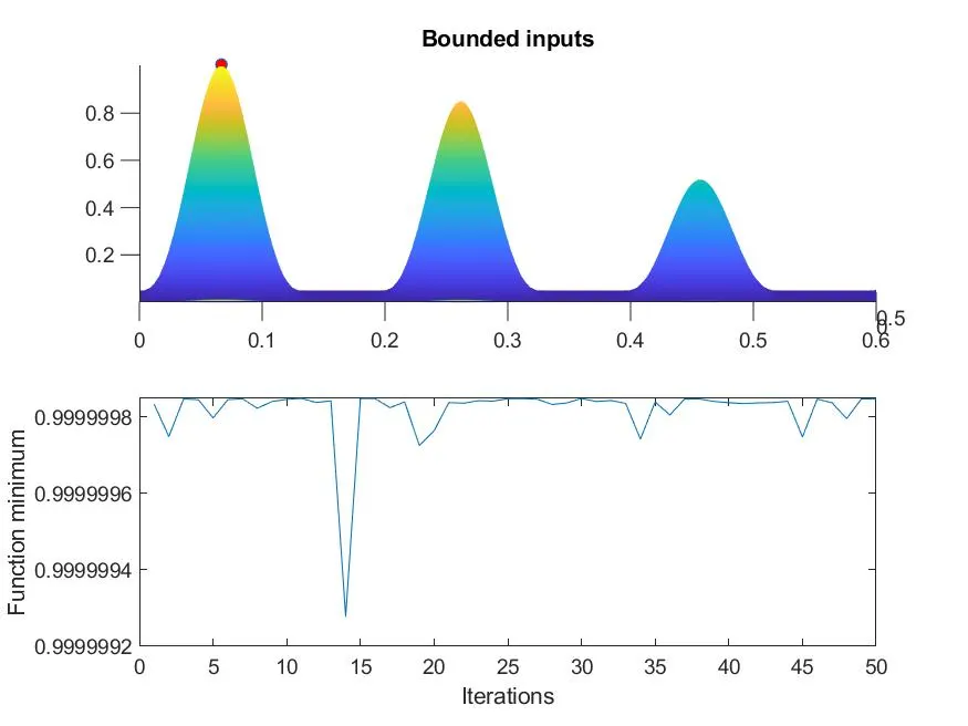
Here population size is 150, so in this case the results are much more reliable and the optimization algorithm are not stuck with local maxima.
We have very slight different outcome each time for the 50 iterations as inputs provided in the program.
RESULTS:-
The above shown is the study of 3 different graphs with the proper code and whatever result is obtained in it is different.
So we make different graphs to visualize all the 3 codes and everything is shown upwards.
We found the proper maxima of the peaks and everything is concluded into it.
CONCLUSION:-
In this program i learnt various new commands and through all these made the code for 3 different graphs.
Use of new commands helped a lot in making the code and outcome of each graph or peaks were different.
REFERENCES:-
(1) https://skill-lync.com/knowledgebase/genetic-algorithm-explained
(2) https://en.wikipedia.org/wiki/Genetic_algorithm
(3) https://www.tutorialspoint.com/genetic_algorithms/genetic_algorithms_introduction.htm