Week 4 - Genetic Algorithm

AIM:

DESCRIBE THE GENETIC ALGORITHM CONCEPT AND IMPLEMENT THE STALAGMITE FUNCTION TO FIND THE GLOBAL MAXIMA USING MATLAB

OBJECTIVE:

• EXPLAIN THE CONCEPTS OF GENETIC ALGORITHM AND STALAGMITE.
• WRITE THE OPTIMIZATION MATLAB CODE FOR STALAGMITE FUNCTION AND FIND THE GLOBAL MAXIMA OF THE FUNCTION.
• EXPLAIN THE SYNTAX OF GENETIC ALGORITHM (ga)
• PLOT THE OUTPUT GRAPH FOR ALL THE STUDIES

THEORY:

1. OPTIMIZATION:

Optimization is a decision-making process, it helps to find the best results. Under a set of prioritized criteria or constraints, it is a procedure which is executed iteratively by comparing various solution till an optimum or a satisfactory solution is found. These include maximizing or minimizing factors such as reliability, efficiency, etc.

2. OPTIMIZATION ALGORITHM:

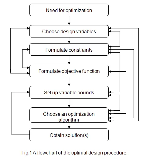
The optimization algorithm contains some parameters like variables, objective function or fitness function, bounding conditions.

3. TYPES OF TECHNIQUES AVAILABLE TO PERFORM OPTIMIzATION:

To perform the optimization there are two types of optimization techniques

• DETERMINISTIC METHOD
• STOCHASTIC METHOD

i. DETERMINISTIC METHOD:

The deterministic method uses specific rules for moving one solution to another. In this technique, the output of the model is fully determined by the parameter values and the initial conditions.

ii. STOCHASTIC METHOD:

The stochastic method is gaining popularity due to certain properties which deterministic algorithm do not possess. The stochastic model process some inherent randomness, it is a probabilistic approach.

4. GENETIC ALGORITHM (ga):

The Genetic algorithm is one of the optimization processes which is simply a stochastic optimization algorithm or search based optimization algorithm. It is based on the mechanisms of natural selection in Charles darwin's theory of natural evolution. It is used to find optimal or sub-optimal solutions. It is frequently used to solve optimization problems in research and machine learning.

5. FORMATION OF GENETIC ALGORITHM:

Genetic Algorithm formation follows the sample data points undergoes the three following steps there are,

a. SELECTION:

In the selection process, the parents are selected from the sample data or random solutions points. The main objective of the selection process is to select the highly fitted individuals, the selection process is taken from Roulette wheel selection, it is also known as Fitness propagation selection it is a genetic operator used in genetic algorithm for selecting a potentially useful solution for recombination.

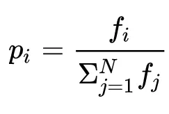
where N is the number of individual in the population

pi is the probability of string, 'i' is being selected

fi is the fitness for string, 'i' in population expressed as f(x)

b. CROSS-OVER:

The crossover is the process of taking two parents' solutions and producing offspring from them. There are many ways to do cross over operation there are one point crossover and multiple point cross over.

c. MUTATION:

The mutation is carried out to maintain the genetic diversity from one generation of a population of chromosomes to the next. If a mutation is not performed the chromosomes will become too similar to each other, Convergence takes place soon and result in local minima similar to the crossover. There are many ways to perform the mutation process there are swap mutation, inverse mutation, etc.

6. WORKING OF GENETIC ALGORITHM:

i). The genetic algorithm starts with an initial set of random solutions called POPULATION.

ii). Each individual in the population is called a CHROMOSOMES which represents a solution to the problem.

iii). Chromosome's values are in the form of a binary system which is 0 and 1.

iv). The chromosomes evolve through successive iterations called GENERATIONS.

v). During each generation, the chromosomes are evaluated using some measures of FITNESS. This fitness is nothing but a value that represents the objective function or fitness value to measure the fitting value.

vi). To create the next generation, new chromosomes have to form which is OFFSPRING.

vii). This offspring can be formed by two methods,

a. Merging two chromosomes from the current generation using a CROSSOVER OPERATOR.

b. Modifying chromosomes using a MUTATION OPERATOR.

viii). A new generation is formed by,

a. Selecting according to the fitness values like some of the PARENTS and OFFSPRING.

b. Rejecting others so that to keep the population size constant.

ix). Fitter chromosomes have higher probabilities of being selected.

x). After several generations, the algorithms converge to the best chromosomes which hopefully represent the optimum or sub-optimal solution to the problem.

xi). When the stopping criteria are obtained then the genetic algorithm will stop the process and have the result of optimal and sub-optimal solutions.

7. STOPPING CONDITIONS :

The genetic algorithm uses the following options to determine when to stop, Where seven stopping conditions are present as follows,

• The algorithm stops as soon as any one of these following conditions is obtained. So in genetic algorithm stopping conditions are so important for stopping criteria to get the minimum value or optimum value.

a. MaxGenerations:

The algorithm stops when the number of generations reaches MAXIMUM GENERATIONS.

b. MaxTime:

The algorithm stops after running for a particular amount of time period in seconds which is equal to the maximum time.

c. FitnessLimit:

The algorithm stops when the value of the fitness function for the best point in the current population is less than or equal to Fitness Limit.

d. MaxStallGenerations:

The algorithm stops when the average relative change in the fitness function value over MaxStallGenerations is less than The Function tolerance.

e. MaxStallTime:

The algorithm stops if there is no improvement in the objective function during an interval of time in seconds equal to MaxStallTime.

f. FunctionTolerance:

The algorithm runs until the average relative change in the fitness function value over MaxStallGenerations is less than FunctionTolerance.

g. ConstraintTolerance:

The ConstraintTolerance is not used as a stopping criterion, but it is used to determine the feasibility with respect to nonlinear constraints. Also, determines feasibility with respect to linear constraints.

8. STALAGMITE:

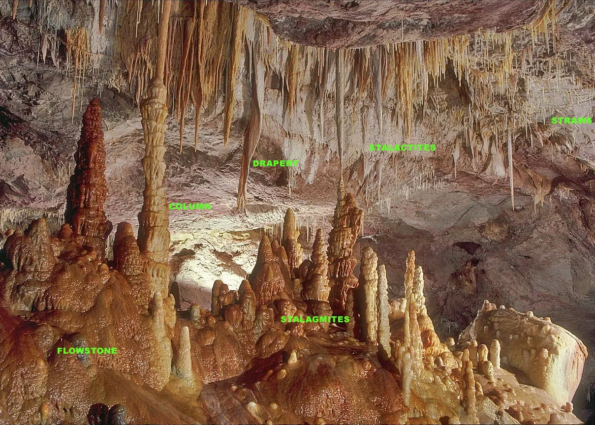
A stalagmite is a type of rock formation that rises from the floor of a cave due to the accumulation of the material deposited on the floor from ceiling drippings. Stalagmites are typically composed of calcium carbonate but may consist of lava, mud, peat, pitch, sand, sinter, and amberat. amberat is the form of crystallized urine of a pack of rats.

9. STALAGMITE FUNCTION:

• Stalagmite function is nothing but an objective function which to calculate the shapes of the stalagmite rock which have global minima and local minima value. Stalagmite function is a measure of the fitness value of the stalagmite shapes.

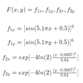
• The above formulas are used to measure the stalagmite shapes

10. GENETIC ALGORITHM SYNTAX :

The genetic algorithm always gives the value of minimal, either global minima or local minima, the syntax to calculate the exact value of global minima can be represented as,

[x, fval] = ga(fun, nvars, A, b, Aeq, beq, lb , ub, nonlcon, IntCon, options)

here the input arguments are,

• fun:

The input argument fun is nothing but an Objective function, specified as a function handle or function name were, the objective function to accept a row vector of length in the number of variables and return a scalar value of the same number of variables.

here, the function handle is denoted as (@), (at the rate of) symbol, it is also to call the function name of the different program to the main program.

Example: x = @get(y) Here get(y) is a separate function program. By giving (@ command we call that particular function program to the main program.)

• nvars:

The input argument nvars is nothing but the number of variables, it is specified as a positive integer. The solver passes row vectors of length, number of variables to the objective function.

• A,b:

A is Linear inequality constraints, specified as a real matrix, A is an M with row by a number of variables of the matrix, where M is the number of inequalities. A encodes the M linear inequalities. A*x <= b, where x is the column vector of the number of variables x(:) and b is a column vector with M elements.

b is Linear inequality constraints, specified as a real vector

If the Linear inequality constraints of the specified real matrix and the vector are not present then the value becomes, set off A = [] and b = [] of a null matrix.

• Aeq,beq:

Aeq is Linear equality constraints, specified as a real matrix, Aeq is an M with row by a number of variables of the matrix, where M is the number of equalities. Aeq encodes the M linear inequalities. Aeq*x = beq, where x is the column vector of the number of variables x(:), and beq is a column vector with M elements.

beq is Linear equality constraints, specified as a real vector

If the Linear equality constraints of the specified real matrix and the vector are not present then the value becomes, set of Aeq =[] and beq = [] of a null matrix.

• lb and ub:

The input argument lb and ub represent the bounding conditions of the lower bounds and the upper bounds.

lb is Lower bounds, specified as a real vector or array of doubles. lb represents the lower bounds element-wise in, lb <= x <= ub. Internally, the genetic algorithm (ga)converts an array lb to the vector lb(:).

ub is Upper bounds, specified as a real vector or array of doubles. ub represents the upper bounds element-wise in, lb <= x <= ub. Internally, the genetic algorithm (ga) converts an array ub to the vector ub(:).

Here, The lower bound and upper bound of x which is optimal value shouldn't exceed the bounding limits of lb and ub values

• nonlcon:

The input argument of nonlcon represents the Nonlinear constraints, it is specified as a function handle or function name. nonlcon is a function that accepts a vector or array x and returns two arrays, which are Linear inequality constraints and Linear equality constraints. Set off nonlcon = [], a null matrix. if no nonlinear constraints exist.

• IntCon:

The input argument of IntCon represents the Integer variables, it is specified as a vector of positive integers taking values from 1 to the number of variables (nvars). Each value in IntCon represents an x component that is an integer value. When IntCon is nonempty then Linear equality constraints of Aeq and beq must be empty which is [] null set, and the Nonlinear constraints nonlcon must return an empty set which is [] null set.

• options:

The input argument of options represents the Optimization options, option command is used to minimize the default optimization parameters replaced by the values in the options

the syntax of the options command is as follows,

options = optimoption(which type of algorithm, option name, initial value)

here option names are like, Constrain Tolerance, PopulationSize, FitnessLimit, etc.

here the output arguments are,

• X:

The output argument of X represents the Solution, where x is the best point that a genetic algorithm located during its iterations or the optimal value where the genetic algorithm is located.

• fval:

The output argument of fval represents the Objective function value at the solution which is x, generally, fval is the function of x which is the function of solution or the optimal point where fval = f(X).

MATLAB PROGRAM FOR SATALGMITE FUNCTION:

• Here get stalagmite input function is the input vector value for stalagmite function.

% calling funtion to stalagmite function as inputs value 
function [f] = get_stalagmite_inputs(x,y)

% 2 dimentional input data
       [xx, yy] = meshgrid(x,y);
       
    
% Evaluating the stalagmite function x amd y values
    for i = 1:length(xx)
        for j = 1:length(yy)
        input_vector(1) = xx(i,j) % row vector of x
        input_vector(2) = yy(i,j) % row vector of y
       f(i,j) = stalagmite(input_vector); 
        end
    end
    
end

• In the stalagmite function, the input vector values are taken from the get_stalagmite function.
• Stalagmite function is an objective function to calculate the fitness value of the optimal or sub-optimal solutions.
• The given formula is to calculate the local and global minima value.

% stalagmite function which is an objective function also known as the fitness function    

function [f] = stalagmite(input_vector)

% calling input values of x and y from get_stalagmite_input function

     x = input_vector(1);
     y = input_vector(2);

% formula for stalagmite rock gobal maximum point in stalagmite.
% here in formula (-1) is to convert the minimum value to maximum value in the objective function.
    
    f1  = (sin(5.1*pi*x+0.5)).^6;
    f11 = (sin(5.1*pi*y+0.5)).^6;
    f2  = exp(-(((4).*log(2))*((x-0.0667).^2))/(0.64));
    f22 = exp(-(((4).*log(2))*((y-0.0667).^2))/(0.64));
    f   = -(f1*f11*f2*f22);

end

1. case study-1 for statistical behavior with no bounding conditions.

1. In case study-1 the Matlab program has no bound conditions.
2. When we don't have a bound condition the genetic algorithm gives a different optimal value for every iteration.
3. Here it takes the value on initial conditions of x and y for 50 cases
4. Here the genetic algorithm is taken for only two variables which are x and y.
5. The get_stalagmite_input(x,y) is the function for input vector values to get the function of the input vector row matrix of x and y inputs.
6. The stalagmite function is an objective function to calculate the fitness value of the solution.
7. The stalagmite function is implemented in ga through function handler which is to call the values for every iteration of ga to get the minimum value.
8. The genetic algorithm always gives the global minimum value or local minimum value, so to find the global maximum value we need to multiply the objective function to (-1) to get the maximum value of global and local positions.
9. Here the ga syntax is simply [x, fval]=ga(@stalagmite, 2), where we take two variables which are x and y.

    clear all
    close all
    clc

% defining our search space inputs
%  one dimential input data
    x = linspace(0,0.6,150)
    y = linspace(0,0.6,150)
    num_cases = 50
% implementing the meshgrid values of x and y    
    
    f = get_stalagmite_inputs(x,y)
   
% study 1 - statistical behavior with no bounding conditions
tic
for i = 1:num_cases
    [inputs fopt(i)] = ga(@stalagmite,2);
    xopt(i) = inputs(1);
    yopt(i) = inputs(2);
   
end
study_1 = toc
figure (1)
subplot(2,1,1)
hold on
surf(x, y, -f)
shading interp
plot3(xopt,yopt,-fopt,'marker','o','markersize',5,'markerfacecolor','r')
title('no bounding conditions')
xlabel('x value inputs')
ylabel('y value inputs')
zlabel('f (global maximum)')
subplot(2,1,2)
plot(-fopt)
title('no bounding conditions')
xlabel('iteration')
ylabel('function minimum')

OUTPUT PLOT AND TIME TAKEN FOR CASE STUDY-1:

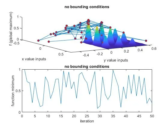
• By seeing the plot we can say that for every iteration we get a different value for optimal solutions of global maximum, so we get different values and case study-1 is a wrong way of approach.
• The main cause we get the value like this is because not having bounding conditions.

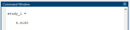
• The output time is taken by using the tic and toc command to know how much time is taken to complete the optimization process for case study-1. The case study time is 4.4160 seconds to complete the iteration or optimal to find the global maximum.

2. case study-2 for statistical behavior in upper and lower bound with bounding conditions:

1. In case study-2 the Matlab program has bound conditions.
2. When we have a bound condition the genetic algorithm gives a different optimal value for every iteration. but the optimal values are present in a particular range limit of lower bound and upper bound which the bound values are given.
3. The lower bound starts from [0 0] and the upper bound ends from [1 1]. in this between the optimal value is found and the values are different for each iteration.
4. Here the ga syntax is simply [x, fval]=ga(fun, nvars, A, b, Aeq, beq, lb, ub), is the syntax for lower bound and upper bound conditions.
5. When the genetic algorithm has Non-Linear inequality constraints and Non-Linear equality constraints, then the values of A and b become empty similarly Aeq and beq becomes empty with a set of [ ] a null matrix value.
6. So in this problem, Linear inequality constraints and Linear equality constraints are not present so the values are zero.
7. Hence the ga syntax changes to [x, fval]=ga(@stalgmite,2,[ ],[ ],[ ],[ ],[0 0],[1 1])
8. Here it takes the value on initial conditions of x and y for 50 cases
9. Here the genetic algorithm is taken for only two variables which are x and y.
10. The get_stalagmite_input(x,y) is the function for input vector values to get the function of the input vector row matrix of x and y inputs.
11. The stalagmite function is an objective function to calculate the fitness value of the solution.
12. The stalagmite function is implemented in ga through function handler which is to call the values for every iteration of ga to get the minimum value.
13. The genetic algorithm always gives the global minimum value or local minimum value, so to find the global maximum value we need to multiply the objective function to (-1) to get the maximum value of global and local positions.

    clear all
    close all
    clc

% defining our search space inputs
%  one dimential input data
    x = linspace(0,0.6,150)
    y = linspace(0,0.6,150)
    num_cases = 50
% implementing the meshgrid values of x and y    
    
    f = get_stalagmite_inputs(x,y)

% study 2 - statistical behavior in upper and lower bound

tic
for i = 1:num_cases
    [inputs fopt(i)] = ga(@stalagmite,2,[],[],[],[],[0 0],[1 1]);
    xopt(i) = inputs(1);
    yopt(i) = inputs(2);
    
end
study_2 = toc
figure (2)
subplot(2,1,1)
hold on
surf(x, y, -f)
shading interp
plot3(xopt,yopt,-fopt,'marker','o','markersize',5,'markerfacecolor','r')
title('bounded condition inputs')
xlabel('x value inputs')
ylabel('y value inputs')
zlabel('f (global maximum)')
subplot(2,1,2)
plot(-fopt)
title('bounded condition inputs')
xlabel('iteration')
ylabel('function minimum')

OUTPUT PLOT AND TIME TAKEN FOR CASE STUDY-2:

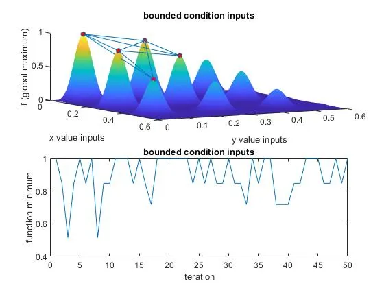
• So compare to case-study-1 the plot changes completely in case-study-2 only because of adding bound conditions.
• Here the optimal values lie's between these 5 peaks were the value of x changes for every iteration, but it won't exceed the bound condition values.
• Here the global maxima are on these 5 peaks, and it still a bit complicated to know the value of global maxima of x.

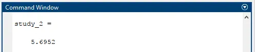
• The output time is taken by using the tic and toc command to know how much time is taken to complete the optimization process for case study-2. The case study time is 5.6952 seconds to complete the iteration or optimal to find the global maximum.

3. case study-3 for statistical behavior with constant population size as options command

1. In case study-3 the Matlab program has bound conditions and options
2. When we have a bound condition and options command the genetic algorithm gives the same optimal value for every iteration.
3. The lower bound starts from [0 0] and the upper bound ends from [1 1]. in this between the optimal value is found and the values are different for each iteration.
4. Here the ga syntax is simply [x, fval]=ga(fun, nvars, A, b, Aeq, beq, lb, ub), is the syntax for lower bound and upper bound conditions.
5. When the genetic algorithm has Non-Linear inequality constraints and Non-Linear equality constraints, then the values of A and b become empty similarly Aeq and beq becomes empty with a set of [] a null matrix value.
6. So in this problem, Linear inequality constraints and Linear equality constraints are not present so the values are zero.
7. Hence the ga syntax changes to [x, fval]=ga(@stalgmite,2,[ ],[ ],[ ],[ ],[0 0],[1 1])
8. With respect to bound conditions by adding the options it helps to minimize the default optimization process to low and we get the accurate value of global maxima.
9. How optimoption command works, option = optimoptions('ga','PopulationSize', 400), where population size is a option name were it has the value of 400. which is the initial population size of 400 random sample solution data.
10. With these individual data samples, the ga going to slow down because it has a large number of population data to calculate to get the global maxima value.
11. When the integer value is non-empty then the Nonlinear constraints must return the value as empty [] set.
12. For option syntax becomes [x, fval]=ga(fun, nvars, A, b, Aeq, beq, lb, ub,nonlcon,IntCon,options)
13. Here intcon and nonlcon are in empty sets off [].
14. So syntax changes as [x, fval]=ga(@stalgnite,2,[ ],[ ],[ ],[ ],[0 0],[1 1],[ ],[ ],option)
15. Here it takes the value on initial conditions of x and y for 50 cases
16. Here the genetic algorithm is taken for only two variables which are x and y.
17. The get_stalagmite_input(x,y) is the function for input vector values to get the function of the input vector row matrix of x and y inputs.
18. The stalagmite function is an objective function to calculate the fitness value of the solution.
19. The stalagmite function is implemented in ga through function handler which is to call the values for every iteration of ga to get the minimum value.
20. The genetic algorithm always gives the global minimum value or local minimum value, so to find the global maximum value we need to multiply the objective function to (-1) to get the maximum value of global and local positions.

    clear all
    close all
    clc

% defining our search space inputs
%  one dimential input data
    x = linspace(0,0.6,150)
    y = linspace(0,0.6,150)
    num_cases = 50
% implementing the meshgrid values of x and y    
    
    f = get_stalagmite_inputs(x,y)

% study 3 - statistical behavior with constant population size as options command
options = optimoptions('ga');
options = optimoptions(options,'PopulationSize',400);
for i = 1:num_cases
    [inputs fopt(i)] = ga(@stalagmite,2,[],[],[],[],[0 0],[1 1],[],[],options);
    xopt(i) = inputs(1);
    yopt(i) = inputs(2);
    
end
study_3 = toc
figure (3)
subplot(2,1,1)
hold on
surf(x, y, -f)
shading interp
plot3(xopt,yopt,-fopt,'marker','o','markersize',5,'markerfacecolor','r')
title('population size constant')
xlabel('x value inputs')
ylabel('y value inputs')
zlabel('f (global maximum)')
subplot(2,1,2)
plot(-fopt)
title('population size constant')
xlabel('iteration')
ylabel('function minimum')

OUTPUT PLOT AND TIME TAKEN FOR CASE STUDY-3:

• So compare to case-study-2 the plot in case-study-3 has only a single global maxima point.
• For every iteration, the value lie's between the optimal value of (0.0668,0.0668)
• By taking the initial large number of population size solution.

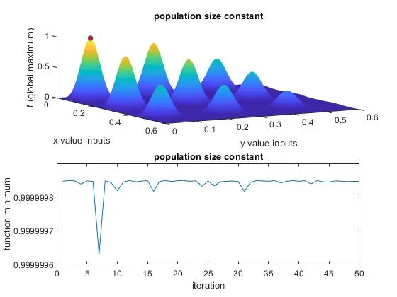
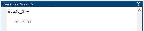
the output time is taken by using the tic and toc command to know how much time is taken to complete the optimization process for case study-3. The case study time is 39.22 seconds to complete the iteration or optimal to find the global maximum.

RESULT:

1. For every iteration, the value of the input lies between point (0.0668,0.0668) of x and y inputs to get global maxima, at present of initial population size at 400. by optimoption command.
2. The genetic algorithm always gives the global minimum value or local minimum value, so to find the global maximum value we need to multiply the objective function to (-1) to get the maximum value of global and local positions.
3. The lower bound starts from [0 0] and the upper bound ends from [1 1]. in this between the optimal value is found and the values are different for each iteration but its in the limit range for that reason bounding condition are used.

REFERANCE:

1. https://skill-lync.com/knowledgebase/genetic-algorithm-explained
2. https://in.mathworks.com/help/gads/how-the-genetic-algorithm-works.html