Project

AIM:

STUDY REPORT ON EXPLAINING HOW TO BUILD AN ALL-TERRAIN VEHICLE (ATV) WITH CONTINUOUSLY VARIABLE TRANSMISSION (CVT) USING BAJA ATV MODEL.

OBJECTIVE:

1. COMPONENTS OF A BAJA ALL-TERRAIN VEHICLE (ATV).
2. VEHICLE MODELING.
   1. DEFINING THE GEAR RATIO.
   2. EFFECT OF PARAMETER VARIATION.
      1. VEHICLE WEIGHT
      2. CVT RATIO
3. INCORPORATING CVT DATA INTO THE MODEL
   1. OPEN-LOOP MODEL
   2. CLOSED-LOOP MODEL

TECHNICAL REPORT:

1. ALL-TERRAIN VEHICLE (ATV):

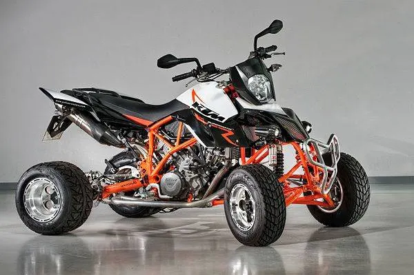
An all-terrain vehicle (ATV), also known as a quad, as defined by the American National Standards Institute (ANSI) is a vehicle that travels on low-pressure tires, with a seat that is straddled by the operator, along with handlebars for steering control. As the name implies, it is designed to handle a wider variety of terrain than most other vehicles

BAJA ALL-TERRAIN VEHICLE (ATV):

Baja is a Collegiate Design Series competition run by the American National Standards Institute(SAE International). Teams of students from universities all over the world, design and build small off-road cars. The cars all have an engine of the same specifications. Baja all-terrain vehicle is an ATV model used in BAJA competition.

COMPONENTS OF A BAJA ALL-TERRAIN VEHICLE (ATV):

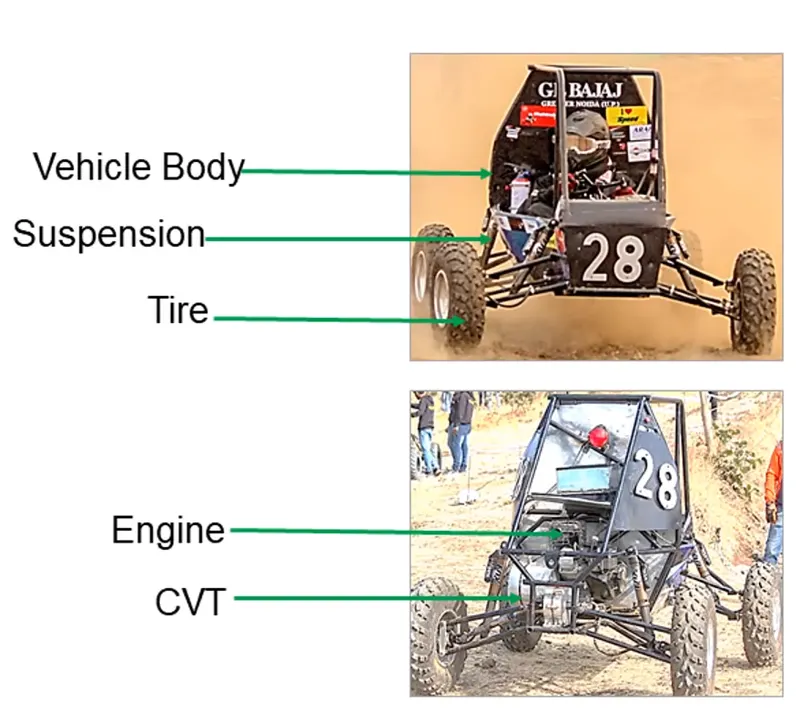
The components of the Baja all-terrain vehicle consists of Vehicle Body, Suspension, Tire, Engine, CVT.

TYPES OF BAJA ALL-TERRAIN VEHICLE (ATV) MODELS:

The Baja AVT model consists of two types there are,

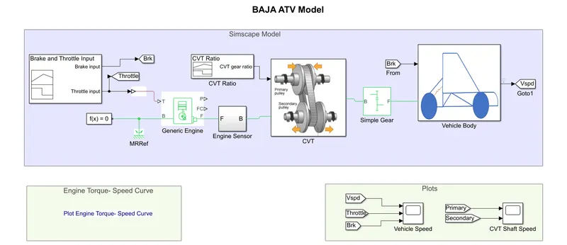
1. SIMULINK MODEL OF BAJA ATV WITH OPEN LOOP CVT MODEL
2. SIMULINK MODEL OF BAJA ATV WITH CLOSED LOOP CVT MODEL

1. SIMULINK MODEL OF BAJA ATV WITH OPEN LOOP CVT MODEL:

2. ENGINE:

In Baja, the ATV is connected to the engine which is a GENERIC ENGINE BLOCK. The Generic Engine Block represents a general internal combustion engine. Engine types included are spark-ignition and diesel. Speed-power and speed-torque parameterizations are provided.

1. Connection T is a Throttle physical signal input that specifies the normalized engine torque.
2. Connections F and B are mechanical rotational conserving ports associated with the engine crankshaft and engine block

THROTTLE:

A Throttle is a mechanism by which fluid flow is managed by constriction or obstruction. An engine's power can be increased or decreased by the restriction of inlet gases, but usually decreased. The term throttle has come to refer, informally, to any mechanism by which the power or speed of an engine is regulated, such as a car's accelerator pedal. What has often termed a throttle is also called a thrust lever, particularly for jet-engine powered aircraft, For a steam locomotive, the valve which controls the steam is known as the regulator.

INPUT THROTTLE CONDITION:

1. The throttle input signal T lies between zero and one and specifies the torque demanded from the engine as a fraction of the maximum possible torque.
2. If the engine speed falls below the Stall speed, the engine torque is blended to zero.
3. If the engine speed exceeds the maximum speed, the simulation stops and issues an error message.

From the signal builder, the throttle conditions are taken initially T as 0.3 for 20 seconds and 1 for 20 to 80 seconds.

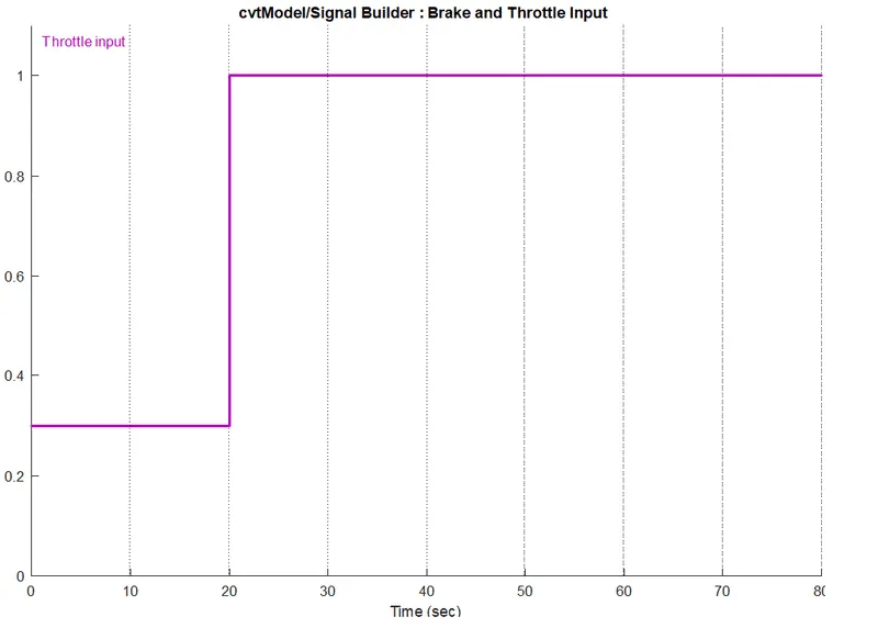
fig -1

BRAKE:

A brake is a mechanical device that inhibits motion by absorbing energy from a moving system. It is used for slowing or stopping a moving vehicle, wheel, axle, or to prevent its motion, most often accomplished using friction

THE BREAK INPUT SIGNAL IS TAKEN AS,

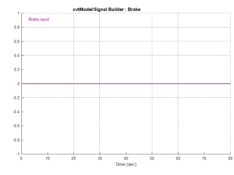
fig-2

FROM fig-3: When we increasing the throttle, the velocity is increasing and after a certain time, it is using the maximum velocity.

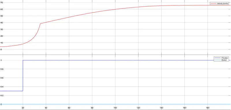
fig-3

SPEED VECTOR AND TORQUE VECTOR INPUT:

The speed vector and Torque vector DATA for the engine are taken from IMAGE DATA which is the Torque Vs Engine speed CURVE.

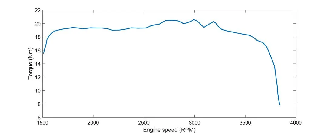
fig -4

To extract the data from the above curve we use one of the file exchangers which is the "GRABIT.m" file.

GRABIT.m:

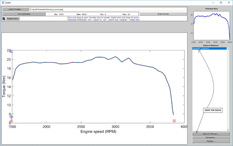
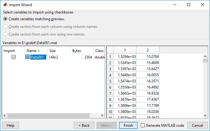
GRABIT is a file exchanger that helps to Extract the data points from an image file. GRABIT starts a GUI program for extracting data from an image file. It is capable of reading in BMP, JPG, TIF, GIF, and PNG files (anything that is readable by IMREAD). Multiple data sets can be extracted from a single image file, and the data is saved as an n-by-2 matrix variable in the workspace. It can also be renamed and saved as a MAT-file.

To extract the data point from GRABIT. First RUN the GRABIT.m file, which opens the GUI program command.

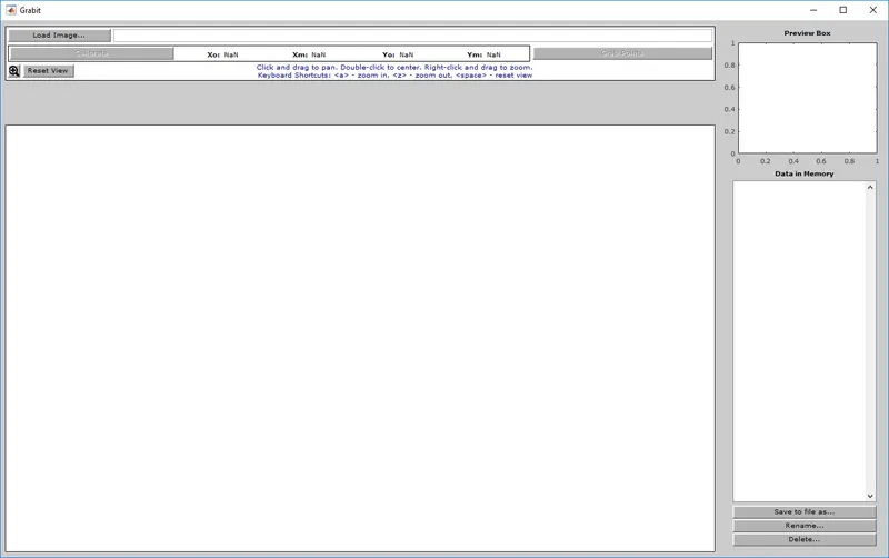
Following steps should be taken:
1. Load the image file.

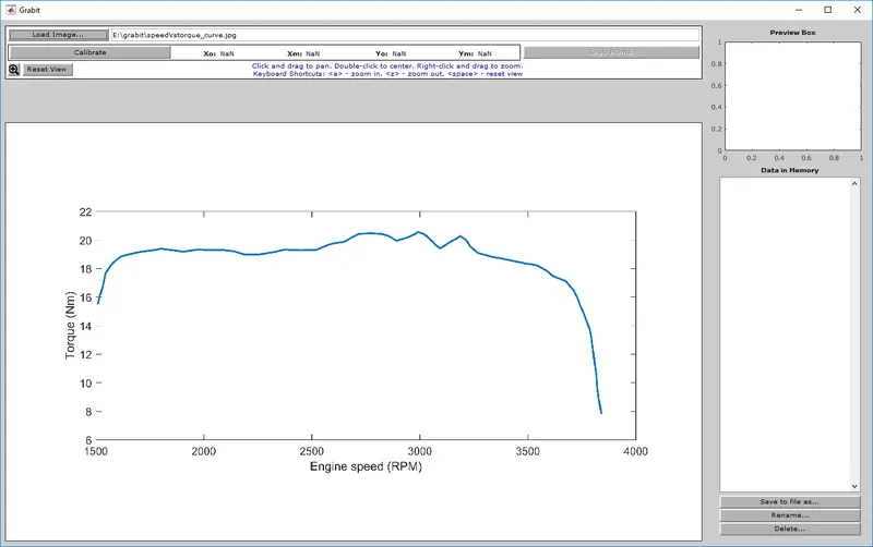
2. Calibrate axes dimensions. You will be prompted to select 4 points on the image.

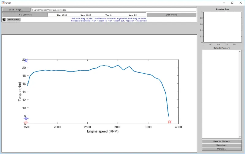
3. Grab points by clicking on points. Right-click to delete a point. The image can be zoomed during this stage.

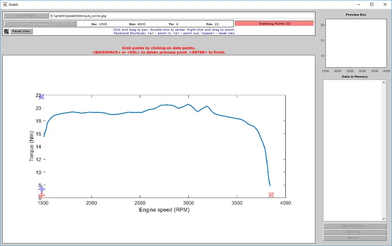
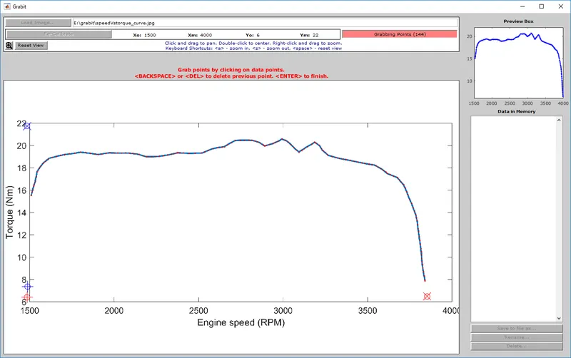
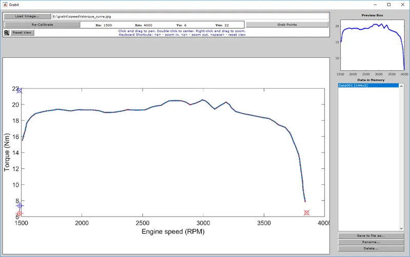
4. Multiple data sets will remain in memory so long as the GUI is open. Variables can be renamed, saved to file, or edited in Array Editor.

1.VEHICLE BODY BLOCK:

The Vehicle Body block represents a two-axle vehicle body in longitudinal motion. The vehicle can have the same or a different number of wheels on each axle. For example, two-wheels on the front axle and two-wheel on the rear axle. The vehicle wheels are assumed identical in size. The vehicle can also have a center of gravity (CG) that is at or below the plane of travel.

The block accounts for body mass, aerodynamic drag, road incline, and weight distribution between axles due to acceleration and road profile. Optionally include pitch and suspension dynamics. The vehicle does not move vertically relative to the ground.

The block has an option to include an externally-defined mass and externally-defined inertia. The mass, inertia, and center of gravity of the vehicle body can vary over the course of simulation in response to system changes.

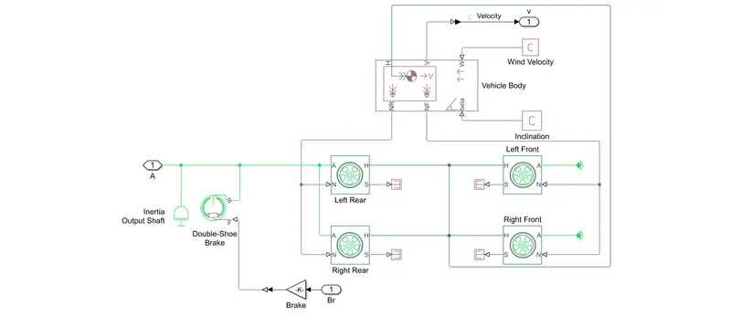
THE SIMULINK OF VEHICLE BODY BLOCK:

1. In this simulation of Vehicle-body is connected to two Rear wheels and two front wheels.
   1. Connection A - is the mechanical rotational conserving port for the wheel axle.
   2. Connection H - is the mechanical translational conserving port for the wheel hub through which the thrust developed by the tire is applied to the vehicle.
   3. Connection N - is a physical signal input port that applies the normal force acting on the tire.
   4. Connection S - is a physical signal output port that reports the tire slip.
   5. Connection V - physical signal output ports for vehicle velocity
   6. Connection NF - physical signal output ports for front normal wheel forces.
   7. Connection NR - physical signal output ports for rear normal wheel forces.
2. Now connection A is connected with Inertia Output Shaft. where inertia output shaft = `1e-1`
3. The Double-Shoe Brake Block The connection S Tire slip is connected to A which is the mechanical rotational conserving port for the wheel axle.

EFFECT OF PARAMETER VARIATION:

VEHICLE WEIGHT:

1. The below fig-5 shows that for every change in Vehicle mass the velocity linearly increases and becomes maximum constant velocity.
2. compare to mass at 100kg the velocity speed is more than 250kg mass velocity
3. The vehicle velocity changes for every mass values

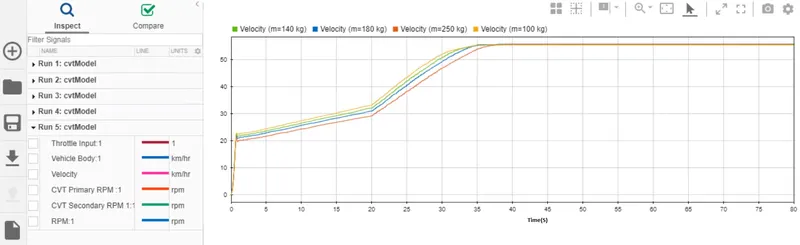
fig-5

3. CVT- CONTINUOUSLY VARIABLE TRANSMISSION:

A continuously variable transmission (CVT) is an automatic transmission that can change seamlessly through a continuous range of gear ratios. This contrasts with other transmissions that provide a limited number of gear ratios in fixed steps. The flexibility of a CVT with suitable control may allow the engine to operate at a constant RPM while the vehicle moves at varying speeds.

CVT is used in automobiles, tractors, motor scooters, snowmobiles, and earthmoving equipment. The most common type of CVT uses two pulleys connected by a belt or chain, however, several other designs have also been used at times.

CVT consists :

mainly CVT consists of, Primary Pulley, Variator, belt, Secondary Pulley.

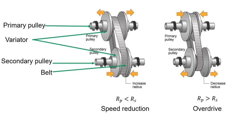
1. The variator which is connected to the Primary Pulley, when it goes out-ward, the variator of Secondary Pulley will move in-ward. Such that the radius of the Secondary Pulley will be more than that radius of the Primary Pulley. So that will lead to SPEED REDUCTION. Which is, `R_p < R_s`
2. The variator which is connected to the Primary Pulley, when it goes in-ward, the variator of Secondary Pulley will move out-ward. Such that the radius of the Secondary Pulley will be less than that radius of the Primary Pulley. So that will lead to OVERDRIVE. Which is, `R_p > R_s`

1. CVT MODEL WITH OPEN LOOP:

OPEN LOOP MODEL:

Inside the CVT block

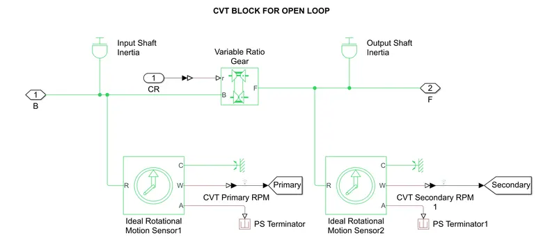
The CVT block consists of,

1. Connection B is connected to Input Shaft Inertia which is a Primary Pulley, where Input Shaft Inertia = `m_1*(((18.6e-2)/2)^2+((2.5e-2)/2)^2)/2`,SI unit is `kg*m^2`.
2. Connection F is connected to Output Shaft Inertia which is a Secondary Pulley, where Output Shaft Inertia = `m_2*(((19.8e-2)/2)^2+((1.9e-2)/2)^2)/2`,SI unit is `kg*m^2`
3. where Connections B (base) and F (follower) are mechanical rotational conserving ports. Specify the relation between base and follower rotation directions with the Output shaft rotates parameter.
4. To specify the CVT ratio we use, the Variable Ratio Gear
5. we get CVT Primary RPM from input shaft inertia and base (B) to the ideal rotational motion sensor-1.
6. we get CVT secondary RPM from output shaft inertia and a follower (F) to the ideal rotational motion sensor-2

EFFECT OF PARAMETER VARIATION:

CVT RATIO:

from fig-6,

1. The range of the CVT ratio is from 0.50 to 3.5, but we know that the range of the CVT ratio is around 0.40 to 3.
2. By taking the value of CVT ratio from 0.5 to 3, the CVT Primary RPM and CVT Secondary RPM varies.
3. When the CVT ratio is Less than 1, the RPM of the primary CVT is greater than the CVT secondary RPM, when it becomes Less than one The secondary RPM is greater than the primary RPM.

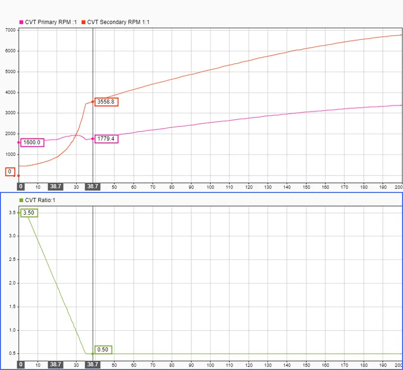
fig -6

From fig-7:

1. The Variation of the Vehicle Velocity curve and CVT's Secondary pulley is almost the same, Reason because The secondary pulley is connected to the rear wheel.

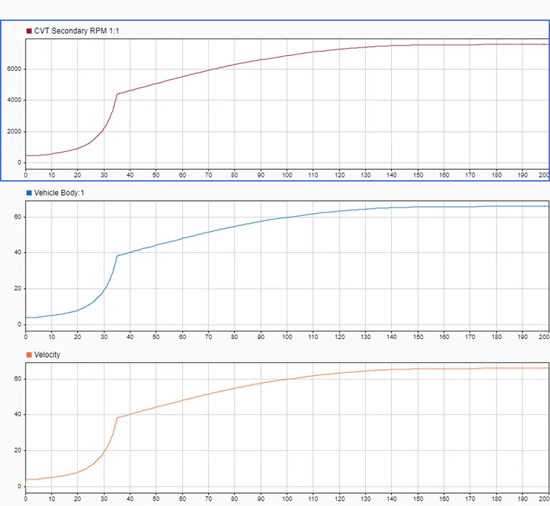
fig -7

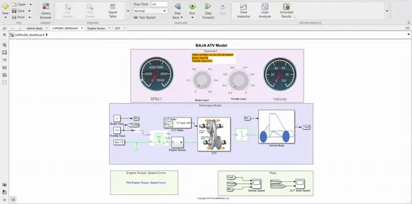
SIMULINK DASHBOARD MODEL OF BAJA ATV WITH OPEN LOOP CVT MODEL:

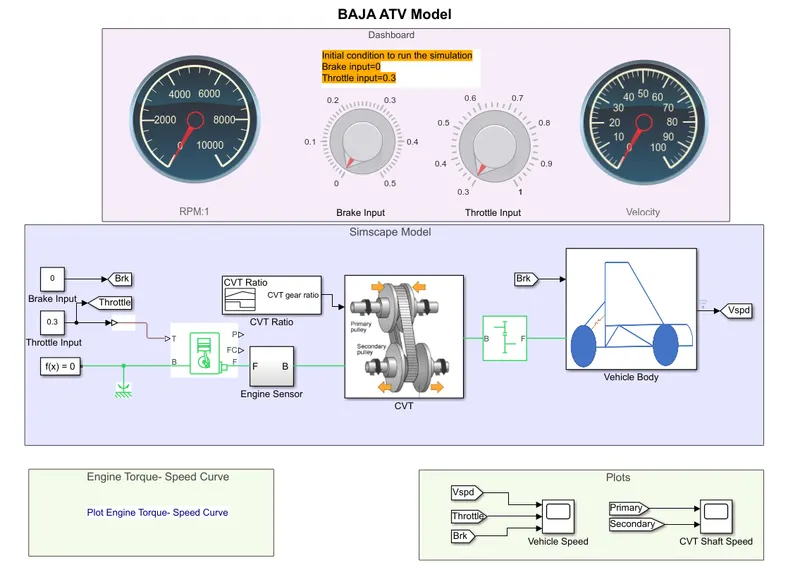
SIMULINK RESULT OF DASHBOARD MODEL OF BAJA ATV WITH OPEN LOOP CVT MODEL:

1. Taking the initial condition for brake at 0 and Trottel input at 0.3 the Engine RPM and Velocity are in running condition.
2. When the Trottel input is gradually increased from 0.3 to 1, the Engine RPM and Velocity values are increased gradually. Similarly, When the Trottel input is gradually decreased from 1 to 0.3, The Engine RPM and velocity values are decreased gradually.
3. When The Brake input is at 0.1 and Trottel at the initial condition at 0.3, the engine rpm and velocity are going to stop suddenly.
4. When Trottel input at a maximum which is at 1 and brake is applied gradually from 0 to 0.5, the Engine RPM and Velocity and gradually coming to rest position or stops.

LIMITATIONS:

The limitation of using the open looped CVT is as follows:

1. In the starting condition of the vehicle, When the Engine RPM and Velocity are in running, it stops the engine RPM and velocity by applying the brakes.
2. In open-loop CVT the problem of facing is stopping or comes to rest quickly.
3. It is not realistic because the CVT ratio has to be depending upon the vehicle velocity, but we Taken the Random CVT values.

2. CVT MODEL WITH CLOSED LOOP:

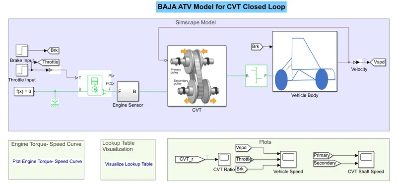
As of now, we have seen that we are giving some random values to the CVT ratio and we are checking the Vehicle performance so, it is not realistic because the CVT ratio is depending upon the vehicle velocity. so, to find the accurate CVT ratio value there is one more model which is the CLOSED-LOOP MODEL.

CVT CLOSED-LOOP MODEL:

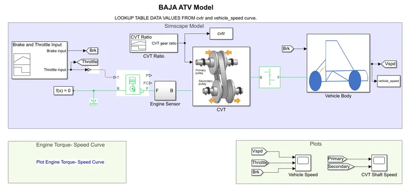
In the closed-loop model, the CVT ratio values are taken from the Vehicle velocity output of the CVT open-loop model by the curve cvtr Vs vehicle speed parameters. The lookup table block readers the data present in the CVT ratio of closed-loop and by implementing the value in CVT block of closed-loop to make a realistic value.

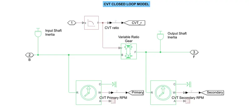
The closed-loop model is built by using LOOKUP TABLE. To get the lookup table value make a written .m file script, where we using the previous CVT open-loop model data and logged the data.

%% Load and simulate the model
cvtModel_data
sim('cvtModel_data')

%% Visualize the lookup table 
plot(vehicle_speed,cvtr,'r','LineWidth',2)
xlabel ('Vehicle Speed (km/hr)')
ylabel ('CVT Ratio')
title ('Lookup Table Visualization')

OPENS PREVIOUS MODEL: getting the values of Vehicle velocity values from the open-loop to closed-loop model through the Lookup table block.

Lookup Table Visualization plot:

The value of the lookup table is taken from the cvtr and Vehicle speed data to a plot we get from the open-loop model of CVT.

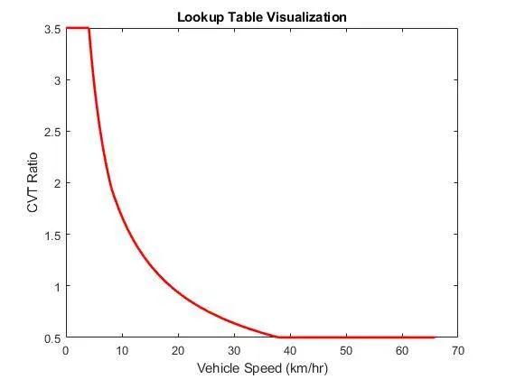
fig-8

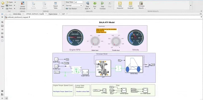
SIMULINK DASHBOARD MODEL OF BAJA ATV WITH CLOSED LOOP CVT MODEL:

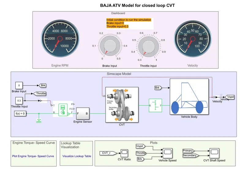
SIMULINK RESULT OF DASHBOARD MODEL OF BAJA ATV WITH CLOSED LOOP CVT MODEL:

1. Taking the initial condition for brake at 0 and Trottel input at 0.3 the Engine RPM and Velocity are in running condition.
2. When the Trottel input is gradually increased from 0.3 to 1, the Engine RPM and Velocity values are increased gradually. Similarly, When the Trottel input is gradually decreased from 1 to 0.3, The Engine RPM and velocity values are decreased gradually.
3. When the Brake input is gradually increased from 0 to 0.5, the Engine RPM and Velocity values are decreased gradually. Similarly, When the Brake input is gradually increased from 0.5 to 0, The Engine RPM and velocity values are increased gradually.
4. When Trottel input at a maximum which is at 1 and brake is applied gradually from 0 to 0.5, the Engine RPM and Velocity values are decreased compared to initial condition but it won't be in stopping condition.

NOTE POINT:

1. By applying the Brakes the engine RPM and Velocity value will become slow down or reduces the speed.
2. The model run in realistic values and real-time data.

RESULT:

1. SIMULINK MODEL OF BAJA ATV WITH OPEN LOOP CVT MODEL:

This model has a problem that whenever we apply the Brakes in running condition the engine stops which RPM at zero and Velocity at zero because it is not realistic because the CVT ratio has to be depending upon the vehicle velocity, but we Taken the Random CVT values.

2. SIMULINK MODEL OF BAJA ATV WITH CLOSED LOOP CVT MODEL:

This model rectifies the problem of Brakes Which are in running conditions by using the realistic data by Depending upon The Vehicle Velocity, so The model is very helpful TO RUN REAL WORLD DATA CONDITIONS.

REFERENCE:

https://in.mathworks.com/matlabcentral/fileexchange/70576-baja-all-terrain-vehicle-atv-model