Week 3 - Solving second order ODEs

AIM:

solving the second-order differential equation using a simple pendulum

OBJECTIVE:

1. Make a plot for Angular Displacement Vs Angular Velocity using MATLAB
2. Create a Simple Pendulum Motion Animation video

THEORY:

• THE NEWTONS SECOND LAW OF MOTION:

Newton's second law states that the rate of change of momentum of a body is directly proportional to the force applied, and this change in momentum takes place in the direction of the applied force.

F=ma

where,

F = the net force applied, kg.m/s²

m = the mass of the body, kg.

a = the body's acceleration, m/s²

• SIMPLE PENDULUM EXPLANATION:

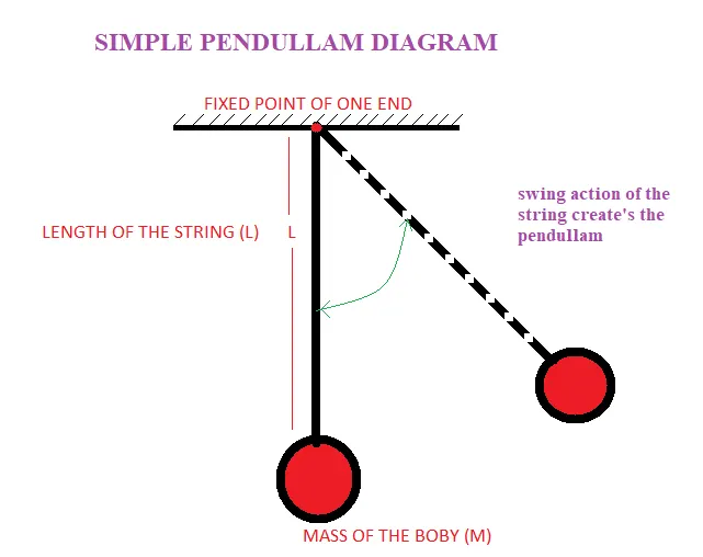
A simple pendulum is a body suspended from a fixed support so that it swings freely back and forth under the influence of gravity. When a pendulum is displaced sideways from its resting, equilibrium position, it is subject to a restoring force due to gravity that will accelerate it back toward the equilibrium position. When released, the restoring force acting on the pendulum's mass causes it to oscillate about the equilibrium position, swinging it back and forth.

The way the pendulum moves depends on Newton's second law. When this law is written down, we get a second order Ordinary Differential Equation that describes the position of the "ball or bob or mass" w.r.t time.

i.e, the equation of the simple pendulum is taken from the Newtons second law of motion

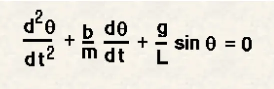
where,

• g = gravity in m/s²
• L = length of the pendulum in m.
• m = mass of the ball in kg.
• b=damping coefficient.

MATLAB PROGRAM:

MAIN PROGRAM

Explanation:

• This program is to create a simple pendulum diagram, making a plot for Angular Displacement Vs Angular Velocity, and creating an avi file of simple pendulum motion video.
• For initial values, length of the string (L) = 1 meter, mass of the ball or bob (m)=1 kg,damping coefficient (b)=0.05, gravity of the body (g)=9.81 m/s2, Timespan is 0-20 sec, angular displacement (t) =0,angular velocity (v) =3 rad/sec at time t=0 is to integration limits from 0 to 20.
• for the value ode_function_of_simple_pendulum(t, theta,l,m,b,g)

% To solve the equation of motion of a simple pendulum with damping using Matlab.

clear all
close all
clc

% intial limites = [Angular displacement(t)=0; Angular velocity(v)=3].
theta_0 = [0;3];

% given inputs.
 l = 1;    % length of the string.
 m = 1;    % mass of the boby or bob in pendulum.
 b = 0.05; % dampping of the body.
 g = 9.81; % gravity of the mass body and string.
 
 % intigration limites of pendulum with 0 to 20 sec.
 t_span = linspace(0,20,200);
 
 % ode_function_simple_pendulum(t,theta,l,m,b,g) is a saperate function call program to calculate diffrential equation.
 
 % commend to slove ode45.
 
 % Angular displacement(t) and Angular velocity(v) are the output result. 
 [t , v] = ode45(@(t,theta) ode_function_of_simple_pendulum(t,theta,l,m,b,g),t_span , theta_0);
 
 % ploting for Angular displacement vs Angular Velocity of an pendulum,for each time value.
 figure(1);
 plot(t,v(:,1));     % plot forAngular displacement for each value of time.
 hold on             % use to create two plot in same plot.
 plot(t,v(:,2))      % plot for Angular Velocity for each value of time.
 axis([0 20 -4 4])   % graph scale position of x and y axis ie,(t,v).
 title('plot for Angular displacement vs Angular Velocity of an pendulum') %plot title.
 xlabel('Angular Displacement (t),sec ')            % x-axis representation.
 ylabel('Angular Velocity (v),rad/sec')             % y-axis representation.
 legend('Angular Displacement','Angular Velocity')  % reprasentation of two different graphs meaning.
 
 % (ct) is nothing but counter were it counts several figures and it shows in the plot.
 
 ct = 1;
 
 % creating pendulum animation.
 
 for i = 1:length(v(:,1))
     
     % calculating x and y coordinates points for a pendulum motion.
     % (x0,y0) points are the fixed point where one end of the pendulum string is fixed.
     
     x0 = 0;
     y0 = 0; 
     
     % (x1,y1) points are motion for pendulum string.
     x1 =  l*sin(v(i,1));
     y1 = -l*cos(v(i,1));
     
     figure(2)
     % creating pendulum motion diagram. 
     plot([x0 x1],[y0 y1],'linewidth',4)  % string diagram.
     hold on
     plot(x1,y1,'o','markersize',15,'markerfacecolor','g') % bob diagram.
     hold on 
    
     % referance axis point
     plot([-1 1],[0 0],'-.','markersize',1)  % x-axis referance line for pendulum motion.
     plot([0 0], [-1 0],'-.','markersize',1) % y-axis referance line for pendulum motion.
     title('pendulum motion animation')      % animation title.
     xlabel('pendulum motion animation')     % animation title.
     ylabel('pendulum motion animation')     % animation title.
    
     % figure reprasentation of animation.
     legend('string or rope','bob or mass','x-axis referance','y-axis referance') 
     axis([-1.5 1.5 -1.5 0.5]) % graph scale position of x and y axis
     pause(0.05)               % speed of the frame that creating
     hold off                  % stoping the figure and presenting all single frames
     % all (ct) frames were stored in array called M and "getframe" command helps to "get current frame" to be plot.
     M(ct)=getframe(gcf); 
     ct = ct+1;                % Incrementing the result of frames or figures.
     
 end
 % creating an avi file.  
 
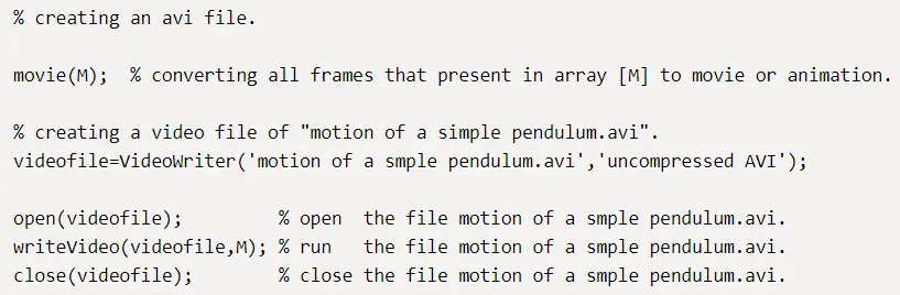
 movie(M);  % converting all frames that present in array [M] to movie or animation.
 
 % creating a video file of "motion of a simple pendulum.avi".
 videofile=VideoWriter('motion of a smple pendulum.avi','uncompressed AVI');
 
 open(videofile);         % open  the file motion of a smple pendulum.avi. 
 writeVideo(videofile,M); % run   the file motion of a smple pendulum.avi.
 close(videofile);        % close the file motion of a smple pendulum.avi.

B. FUNCTION PROGRAM:

• Explanation:

the second order diffrential equation of (d^2theta_dt^2) gives two outputs, to caluclate the two outputs (d^2theta_dt^2) will splite in to two equations they are dtheta1_dt and dtheta2_dt.

now,

• dtheta1_dt = theta2; this is equation 1
• dtheta2_dt = -(b/m)*theta2 - (g/l)*sin(theta1); this is equation 2

By solving the above equation dtheta1_dt and dtheta2_dt we get dtheta_dt which is an output value of (d^2theta_dt^2)

to call this function values in main program (ode45) command is very useful to calculate the differential equations

% function to solve the second-order equation, an ode
        
% function output is dthet_dt.
% function inputs are t,theta,length of string,mass,damping,gravity of the mass.

function [dtheta_dt] = ode_function_of_simple_pendulum(t,theta,l,m,b,g)
         
         theta1 = theta(1);  % for every theta1 value its storeing in theta(1).  
         theta2 = theta(2);  % for every theta2 value its storeing in theta(2).
        
         % second order differential equation has to brake in to two equation.
         % dtheta1_dt is the first equation.
         % dtheta2_dt is the second equation.
         dtheta1_dt = theta2;    
         dtheta2_dt = -(b/m)*theta2 - (g/l)*sin(theta1);
         % disply in the valus of two equation in main pogram.
         dtheta_dt = [dtheta1_dt; dtheta2_dt];
         
end
         
       % END RESULT VALUES WILL CALL FROM MAIN PROGRAM ie, the motion of a simple pendulum.

C. ODE 45 COMMAND:

ODE45 is a mathematical expression to solve the differential equation, basically, ODE solves any type of orders to calculate, simple or complex expression. in this program to calculate the differential equation first output variables to be given that is [t, v] are angular displacement and angular velocity, followed by ode45 command with windows handler to calculate the input value which is time (t) and theta values, ode_function_of_simple_pendulum(t, theta,l,m,b,g) is a separate function program to calculate the (theta) value. with integral of t_span which is 0 to 20 values and theta_0 are final limits of 0 and 3 of data.

program for creating Simple Pendulum Motion Animation video:

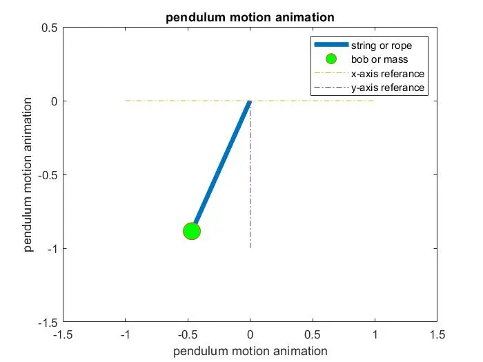
1. program that creates a string diagram using linewidth command

In this program one end of the pendulum string is fixed that is (x0, y0) points and the length of the string endpoint is taken as (x1, Y1). By using the linewidth command the width of the string expands to 4 mm,

the length of the string is 1m.

2.program that creates ball or bob diagram using marker command

In this program, the endpoint of (x1, Y1), we create a ball using the marker command with the ball size is 15mm, and the color of the ball is green.

3.program that creates reference points of the x-axis as a fixed point and y-axis as motion points using marker command.

In this program, we explain the swing action of the pendulum reference axis from one coordinate axis to other coordinates axis. by using the marker command of ('-.') we create a dotted line.

4.program that creates the animation or avi file:

The below program helps to create the video file or avi.file for simple pendulum motion animation. movie(M) will do converting all frames that present in array [m] to make a video. where M is several frames that are created per second. VideoWriter commend helps to create the video file name and profile name for the particular video. writeVideo command help to create the animation video by using the data of video file name and frames that created in M array.

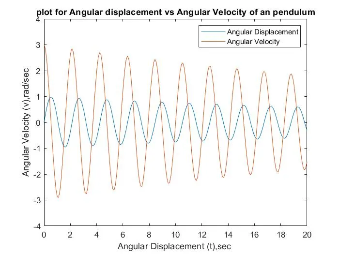
OUTPUT PLOTS FOR ANGULAR DISPLACEMENT Vs ANGULAR VELOCITY:

The plot shows wave motion of angular displacement and angular velocity, for each time span of 0 to 20 were angular velocity is higher than the angular displacement.

SIMPLE PENDULUM DIAGRAM CREATED USING MATLAB:

Diagram explanation:

for every time period 0 to 20, angular displacement and angular velocity changes with theta angles. we created a pendulum diagram.

LINK FOR OUTPUT:

Simple Pendulum Motion Animation video link-title

https://youtu.be/rMjgoiM5olo