Genetic Algorithm
Aim:
To optimise the stalagmite function and to determine the global maxima of the given search space.
Objectives:
- To optimise the stalagmite function.
- To plot the values obtained from the stalagmite function.
- To determine the global maxima of the given workspace.
Genetic Algorithm:
Genetic algorithm (GA) is inspired by the process of natural selection. Genetic algorithms are commonly used to generate high-quality solutions to optimization and search problems by relying on biologically inspired operators such as mutation, crossover and selection. The genetic algorithm selects a set of random samples within the given boundary conditions, options for the set of data or function and the data itself. A portion of the existing population is selected to breed a new generation. Individual solutions are selected through a fitness-based process, where fitter solutions (as measured by a fitness function) are typically more likely to be selected. For each new solution to be produced, a pair of "parent" solutions are selected for breeding from the pool selected previously. By producing a "child" solution using crossover and mutation, a new solution is created which typically shares many of the characteristics of its "parents". New parents are selected for each new child, and the process continues until a new population of solutions of appropriate size is generated. These processes provide a solution which is way too different from the initial set of parent data. The process ends after a solution that satisfies the minimum criteria are obtained or a fixed number of generations is reached or through manual inspection.
The syntax for ga in MatLab is as follows:
x = ga(fun,nvars,A,b,[],[],lb,ub,nonlcon,IntCon,options)
x = ga(fun,nvars)
where x is the output variable and function refers to the set of data that needs to be optimised through the given function. A b refers to the linear inequalities present in the function. lb and ub are the lower and upper bounds for the given search space and nonlcon refers to the non-linear constraints and intcon refers to the integer constraint. Options are other contains like the size of iterations.
Stalagmite function is a mathematical model that helps to generate maximas and minimas. Global maxima is a maximum peak value in the entire function and global minima is a minimum peak value in the entire function. But local maxima and local minima are multiple numbers of values. The Stalagmite function is as follows:
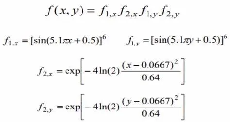
The negative sign is used to determine the maximum value as the stalagmite function and ga solver mainly works on optimizing the results to the minimum value.
Code:
Stalagmite Function Part:
function [fx_y] = stalgamite(in_vector)
x = in_vector(1);
y = in_vector(2);

f1_x = (sin((5.1*pi.*x)+0.5))^6;
f1_y = (sin((5.1*pi.*y)+0.5))^6;
f2_x = exp((-4*log(2)).*(((x-0.0667)^2)/0.64));
f2_y = exp((-4*log(2)).*(((y-0.0667)^2)/0.64));

fx_y = -(f1_x.*f2_x.*f1_y.*f2_y); %Stalagmite function
end
Main Program:
clear all;
close all;
clc;

%Defining the search space
x = linspace(0,0.6,200); %creates 200 divisions between 0 and 0.6
y = linspace(0,0.6,200);

%creating a meshgrid
[xx yy] = meshgrid(x,y); %creates 200*200 matrix

%evaluating the Stalgamite function
for i = 1:length(xx)
    for j = 1:length(yy)
        in_vector(1) = xx(i,j); %copies x values to in_vector array
        in_vector(2) = yy(i,j); %copies y values to in_vector array
        f(i,j) = stalgamite(in_vector);
    end
end

figure(1)
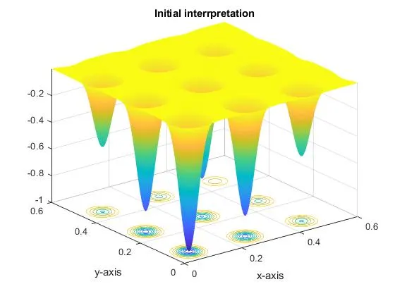
surfc(xx,yy,f) %creates surface plot for x,y and stalagmite function values
xlabel('x-axis');
ylabel('y-axis');
title('Initial interrpretation');

shading interp

[inputs, fval] = ga(@stalgamite,2); %initialise ga function and assigning the optimal
                                    %values to the inputs


%Study-1 Statistical behaviour
num_cases = 50; %perform the ga for 50 iterations

for i = 1:num_cases
    [inputs1, fopt(i)] = ga(@stalgamite, 2);
    xopt(i) = inputs1(1); %assigns the x values of inputs1 to xopt
    yopt(i) = inputs1(2); %assigns the y values of inputs1 to yopt
end

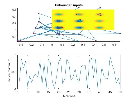
figure(2)
subplot(2,1,1)
hold on
surfc(x,y,f)
shading interp
plot3(xopt,yopt,fopt,'marker','o','markersize',4,'markerfacecolor','r') %marks opt pts
title('Unbounded inputs')
subplot(2,1,2)
plot(fopt)
xlabel('Iterations');
ylabel('Function maximum');


tic
%Study-2 Statistical behaviour - with upper and lower bounds
for i = 1:num_cases
    [inputs1, fopt(i)] = ga(@stalgamite,2,[],[],[],[],[0;0],[1;1]);
    xopt(i) = inputs1(1);
    yopt(i) = inputs1(2);
end
study2_time = toc %time taken for 50 cases with upper and lower bounds

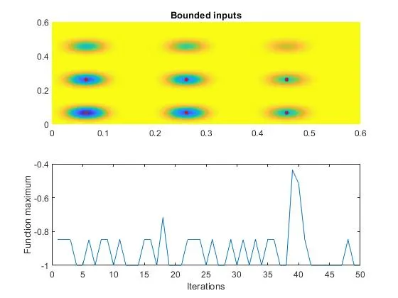
figure(3)
subplot(2,1,1)
hold on
surfc(x,y,f)
shading interp
plot3(xopt,yopt,fopt,'marker','o','markersize',4,'markerfacecolor','r')
title('Bounded inputs')
subplot(2,1,2)
plot(fopt)
xlabel('Iterations');
ylabel('Function maximum');

%Study-3 increasing GA iterations
options = optimoptions('ga'); %creates optimal options for ga
options = optimoptions(options,'PopulationSize',300); %provides 300 iterations as size

tic
for i = 1:num_cases
    [inputs1, fopt(i)] = ga(@stalgamite,2,[],[],[],[],[0;-1],[0.5;0.5],[],[],options);
    xopt(i) = inputs1(1);
    yopt(i) = inputs1(2);
end
study3_time = toc

figure(4)
subplot(2,1,1)
hold on
surfc(x,y,f)
shading interp
plot3(xopt,yopt,fopt,'marker','o','markersize',4,'markerfacecolor','r')
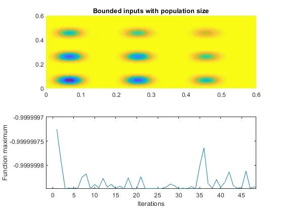
title('Bounded inputs with population size')
subplot(2,1,2)
plot(fopt)
xlabel('Iterations');
ylabel('Function maximum');
Explanation:
The function part of the code is where the search space array as provided and is turned into a set of data with the help of stalagmite function. It is then passed to the ga to determine the optimal solution. Initial surface plot is made to provide a basic outlook for local maxima peaks. As the ga works on random sampling, the results obtained are randomised at every single time. So, a number of iterations, in here 50 is taken and ga is performed. Their optimum x and y values at each iteration are assigned into an array and a plot is made. To improve the results and reduce the randomness, upper and lower bounds are provided so that it could provide the best possible result. To improve the effectiveness of the solution, option command is used to provide an optimised option for ga with the size of 300. The ga is performed with bounds and the options which provided the best possible result and reduced the randomness of the optimal value obtained.
Results:
Conclusion:
Ga can be used to determine the optimal solution (maximise and minimise) based on the objective of the problem and the randomness of the value obtained can be controlled by adding boundary conditions, iterations and the size for optimal options.
References:
https://en.wikipedia.org/wiki/Genetic_algorithm
https://in.mathworks.com/help/
Matlab Documentation
Links:
https://drive.google.com/file/d/1HnyN7wF6AWwV3SSo7rq3UEzGjoQWbPKa/view?usp=sharing
https://drive.google.com/file/d/1Ql9RWU2L329Cb5PMjiN25h6dX0RoHVEf/view?usp=sharing
https://drive.google.com/file/d/17Hh9svWepGuV4muIXDmVhX7eOBnM3Zr4/view?usp=sharing
https://drive.google.com/file/d/1-rd-CU-kL3DA65lrnf92dXu8YDG6UZDn/view?usp=sharing
https://drive.google.com/file/d/1YGCytd_-UYD7v8491ZgCg9VYCKBNtr6X/view?usp=sharing
https://drive.google.com/file/d/1ilfZpUxoBTNjyt3Kv0hFjFH3KkR07VQr/view?usp=sharing
https://drive.google.com/file/d/1vfca9LeuS-pEoKlt_ZNB2Yf3j_WlAwqb/view?usp=sharing