Solving second order ODE (damped pendulum oscillation)

Aim:

The main idea of this project is to create a program for the given system (pendulum with the damper in this case) and to animate the motion of the pendulum.

Objectives:

1. To create a MATLAB program for the given ODE.
2. To animate the given ODE.

Theory:

An ordinary differential equation is a type of differential equation that contains one or more functions of an independent variable with its derivatives. Differential equations are useful for creating and solving a system. Starting from a simple pendulum to structural analysis of huge complex bodies, a differential equation breaks down the problem into smaller elements that may be of an ODE or partial differential equation to solve the element and it can be integrated to solve the problem on the whole. It has a variety of application in Finite element analysis, waves and oscillation/Harmonics and so on.

The equation to be solved (ordinary differential equation):

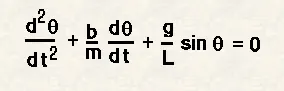
Here, the differential equation is based on the function of `theta` and its derivatives. `theta` is the angular displacement of the pendulum. b is the damping coefficient of the damper. m refers to the mass of the bob hanging and L refers to the length of the string. This provides a general equation for the motion of a pendulum with respect in the form of angular acceleration, velocity and displacement over a period of time.

CODE:

Function part of the code:

function [dtheta_dt]=ode_func(t,theta,b,g,l,m)

theta1=theta(1);
theta2=theta(2);
dtheta1_dt=theta2;
dtheta2_dt=(-(b/m)*theta2)-((g/l)*sin(theta1));
dtheta_dt=[dtheta1_dt; dtheta2_dt];

end

Main code(plotting and animation of the pendulum's angular displacement):

clear all;
close all;
clc;

%input variables
l=1; %l refers to the length of the string in metre
m=1; %m is the mass of the bob in Kg
b=0.05; %b is the damping coefficient
g=9.81; %g refers to the acceleration due to gravity in m/s^2

%initial condition
theta_0=[0;3];  
%Its of 2 rows and one column where the element 1 is angular 
%displacement and the second element is the angular velocity at time 0 sec

%timespan
t_span=linspace(0,20,1000); %refers to the time span of 20 sec with 1000 intervals 

[t,results]=ode45(@(t,theta) ode_func(t,theta,b,g,l,m),t_span,theta_0);

%calls the inbuilt ODE solver in MatLab

%ploting
figure(1)
plot(t,results(:,1)) %plots graph for angular displacement and time
hold on
plot(t,results(:,2)) %plots graph for angular velocity and time
grid on
xlabel('time')
ylabel('plot')
legend('angular displacement','angular velocity');

%animation

ct=1;   %frame counter
for i=1:length(results(:,1)) 
%for 1000 values over time of 20 sec we are plotting an individual graph
    
    x0=0;
    y0=0;
    x1=-(l*sin(results(i,1)));
    y1=-(l*cos(results(i,1)));
    
    figure(2)
    plot([x1,x0],[y1,y0],'linewidth',3)
    axis([-2 2 -1.5 1.5]);
    viscircles([0 0],0.02);
    viscircles([x1 y1],0.1);
    axis off
    
    M(ct)=getframe(gcf); %gets individual plots as frames
    ct=ct+1;             %moves to the next frame
   
end

movie(M)
videofile=VideoWriter('pendulum_motion','Uncompressed AVI'); 
%provides video name and type
open(videofile) %opens the videofile
writeVideo(videofile,M)
close(videofile)

Explanation:

The function part of the ode has the main equation that needs to be solved. Coming to the main program, the input parameters like the length of the string, the mass of the bob, damping coefficient, acceleration due to gravity, the time span and the required intervals are given along with the initial conditions of the angular displacement and velocity at 0 sec. the linspace command generates 1000 values from 0 to 20 and to get the results for the angular velocity and acceleration at that interval of time, the matrix is assigned to the ODE45 solver in MatLab based on the syntax. The code calls the ode function to solve for angular displacement and velocity at every value of time t. A plot is made between the magnitude of angular displacement and time as well as for the magnitude of angular acceleration and time. That gives us an idea of how effective the damper is and the time required for the pendulum to attain an equilibrium position.

For the animating the motion of the pendulum, we already have the results for angular displacement at every value of time t. so we can use a FOR loop for 1000 obtained values and create individual plots. The plots in here known as frames are counted by variable ct which is used to allocate every frame to the array M. Those frames are then written into the video file (here it is the pendulum motion which is assigned to the videofile variable).

Output:

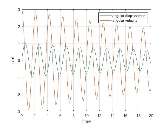
The above graph provides an idea of how damping works in reducing the oscillation of a pendulum over a period of time. As the damping coefficient, in this case, is small in magnitude, we are unable to find a drastic change in angular displacement and velocity. This also provides that the length of the string, time interval, the damping coefficient plays a major role in the way that the pendulum oscillates.

Video and program links:

https://drive.google.com/file/d/1IqCYlXtS8_Y8iCJkZ_FB_VE0NH04EZrl/view?usp=sharing

https://drive.google.com/file/d/1e3pmX7adURN55NTy5EnMFKsvqnPD502J/view?usp=sharing

https://drive.google.com/file/d/1RayHZEZ6QY6gjLGQWT0AeEDK7IHG_JrQ/view?usp=sharing

https://drive.google.com/file/d/1EBY8mE084J2EZi__4GB8ADy6mzfL31Yc/view?usp=sharing