Week 4 - Genetic Algorithm

Optimizing the Stalagmite function using Genetic Algorithm in MATLAB.

Aim

To write a program in MATLAB which optimizes the Stalagmite function and thereby determining the function maxima using Genetic Algorithm ('ga') solver.

Approach to the code

Several blogs, articles, videos and websites were referred to understand the concept of genetic algorithm and how it is used as a search method to determine the optimum value.

Concept of Genetic Algorithm

Genetic Algorithm is a heuristic search based algorithm that is based on the Theory of Natural Selection by Charles Darwin.

It is frequently used to find optimal or near-optimal solutions to difficult problems which otherwise would take a lifetime to solve. It finds application in solving optimization problems, in research, and in machine learning.

The flow chart below gives a general idea of how genetic algorithm works

The process of natural selection starts with the selection of fittest individuals from a population. They produce offspring which inherit the characteristics of the parents and will be added to the next generation. If parents have better fitness, their offspring will be better than parents and have a better chance at surviving. This process keeps on iterating and at the end, a generation with the fittest individuals will be found.

The process starts with a set of individuals from a population. An individual is characterized by a set of parameters (variables) known as Genes. Genes are joined into a string to form a Chromosome (solution).

The fitness function determines how fit an individual is to be selected for reproduction with another individual. In our case, the fitness function is given by the stalagmite function in our case.

• The idea of selection phase is to select the fittest individuals and let them pass their genes to the next generation.
• Crossover is the most significant phase in a genetic algorithm. For each pair of parents to be mated, a crossover point is chosen at random from within the genes. Offsprings are created by exchanging genes from parents until crossover point is reached. These new individuals are added to the population.
• In some new offspring formed, some of their genes can be subjected to a mutation with a low random probability. This implies that some of the bits in the bit string can be flipped. Mutation maintains diversity in the population to avoid premature convergence.
• The algorithm terminates if the population has converged (does not produce offspring which are significantly different from the previous generation). Then it is said that the genetic algorithm has provided a set of solutions to our problem.

This basic concept is applied in Optimization problems to arrive at its maxima and minima which otherwise would take years to solve.

Syntax for ga

Three syntaxes for genetic algorithm were used in this particular program.

x = ga(fun,nvars)
x = ga(fun,nvars,A,b,Aeq,beq,lb,ub)
x = ga(fun,nvars,A,b,Aeq,beq,lb,ub,nonlcon,options)

where fun is the function code that needs to be called

nvars is the number of variables.

A, b represent the linear inequalities and Aeq, beq represent linear equalites.

lb, ub are lower and upper bounds.

nonlcon take in non linear constraints as input.

options calls the options array which contains any modifications made to the syntax.

[] are set if any of these inputs are unknown.

Function code to run the Stalagmite function

ga in MATLAB requires a function code in its syntax and therefore the objective function (stalagmite function in this case) is entered as a function code.

The function definitions for the Stalagmite function are entered as code for both x and y variables.

The output is stored under the function name stalagmite_func.

%function for Genetic_algorithm
function [stalagmite] = stalagmite_func(input_vector)

x = input_vector(1);
y = input_vector(2);

%function definitions
f1x = [sin(5.1*pi*x + 0.5)]^6;
f1y = [sin(5.1*pi*y + 0.5)]^6;

f2x = exp (-4*log(2)*(x-0.0667)^2/(0.64));
f2y = exp (-4*log(2)*(y-0.0667)^2/(0.64));

[st] = [f1x*f1y*f2x*f2y]; 
[stalagmite] = -[st];  %negation in order to obtain the maxima while running ga

end 

Since ga determines the minima of a function by default, (-) is included with the function in the objective function code to obtain the maxima.

Code for the Stalagmite function

The Stalagmite function is entered as code initially, for ease of representation.

Code begins with clear all, close all and clc commands.

The inputs variables of x and y are entered using the linspace commands.

The number of cases which denotes the number of iterations is also entered.

A 2-Dimensional mesh [xx yy] for the x and y variables is created using the meshgrid command.

for loop is then used to call in all the variables from the [xx yy] array. The input vector(1) and input vector(2) contains the xx and yy variables respectively.

These values are then sent into the function for computation.

clear all
close all
clc

%inputs
x = linspace(0,0.6,150);
y = linspace(0,0.6,150);
number_cases = 50;

%Creating a 2D mesh for the x and y values
[xx yy] = meshgrid(x,y);

for i = 1:length(xx);
    for j = 1:length(yy);
        input_vector(1) = xx(i,j);
        input_vector(2) = yy(i,j);
        f(i,j) = stalagmite_func(input_vector);       
    end
end

The reason we use input_vector to store both x and y values as one array is because the ga syntax requires the input of variables as a single array.

Study-1

The first study is to check the statistical behavior of the Genetic algorithm.

The ga command is entered using the ga(fun,nvars) syntax. @ is used to call the function as an anonymous function. 2 is the number of variables.

tic and toc is used to check the time elapsed between start and end of the search.

% Study 1 - Statistical behaviour of the genetic algorithm running this function. 
tic
for i = 1:number_cases
    [inputs ,fopt(i)] = ga(@stalagmite_func,2);
    xopt(i) = inputs(1);
    yopt(i) = inputs(2);
end
Time_taken_study_1 = toc

Result for Study-1

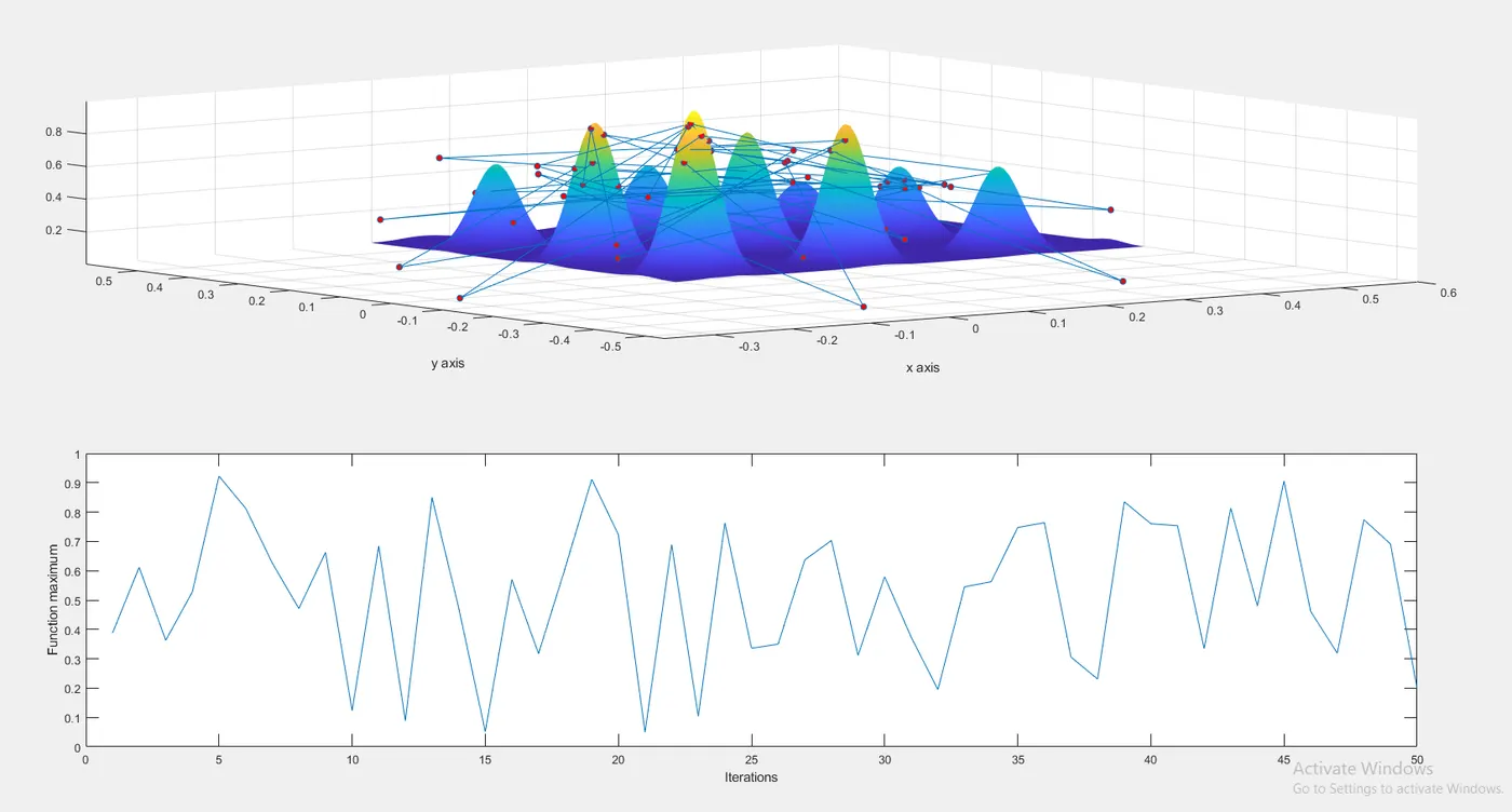
• It can be observed from the first study that the ga produces different function maximum with each iteration. (i.e) the search leads to several outputs that the ga concludes as optimum.
• Study - 1 goes to show that either the population size has to be increased or upper and lower bounds need to be provided to narrow down the search space.
• The variation is denoted more clearly in the second subplot.
• The time taken to run the ga for study - 1 was 4.95 seconds.

Study - 2

The second study is done with the genetic algorithm by providing upper bounds and lower bounds.

The syntax which requires the input of upper and lower bounds is used in this case.

The search space was bound to 0-0.5 in the x-axis and 0-0.5 in the y-axis initiallly.

Upon observing the resultant graph, the optimum values were varying with a lower range.

So the upper and lower bound range was reduced to narrow down the space.

%Study 2 - Genetic algorithm search using upper and lower bounds
tic
for i = 1:number_cases
    [inputs ,fopt(i)] = ga(@stalagmite_func,2,[],[],[],[],[0,0],[0.3,0.3]);
    xopt(i) = inputs(1);
    yopt(i) = inputs(2);
end
Time_taken_study_2 = toc

Result for Study - 2

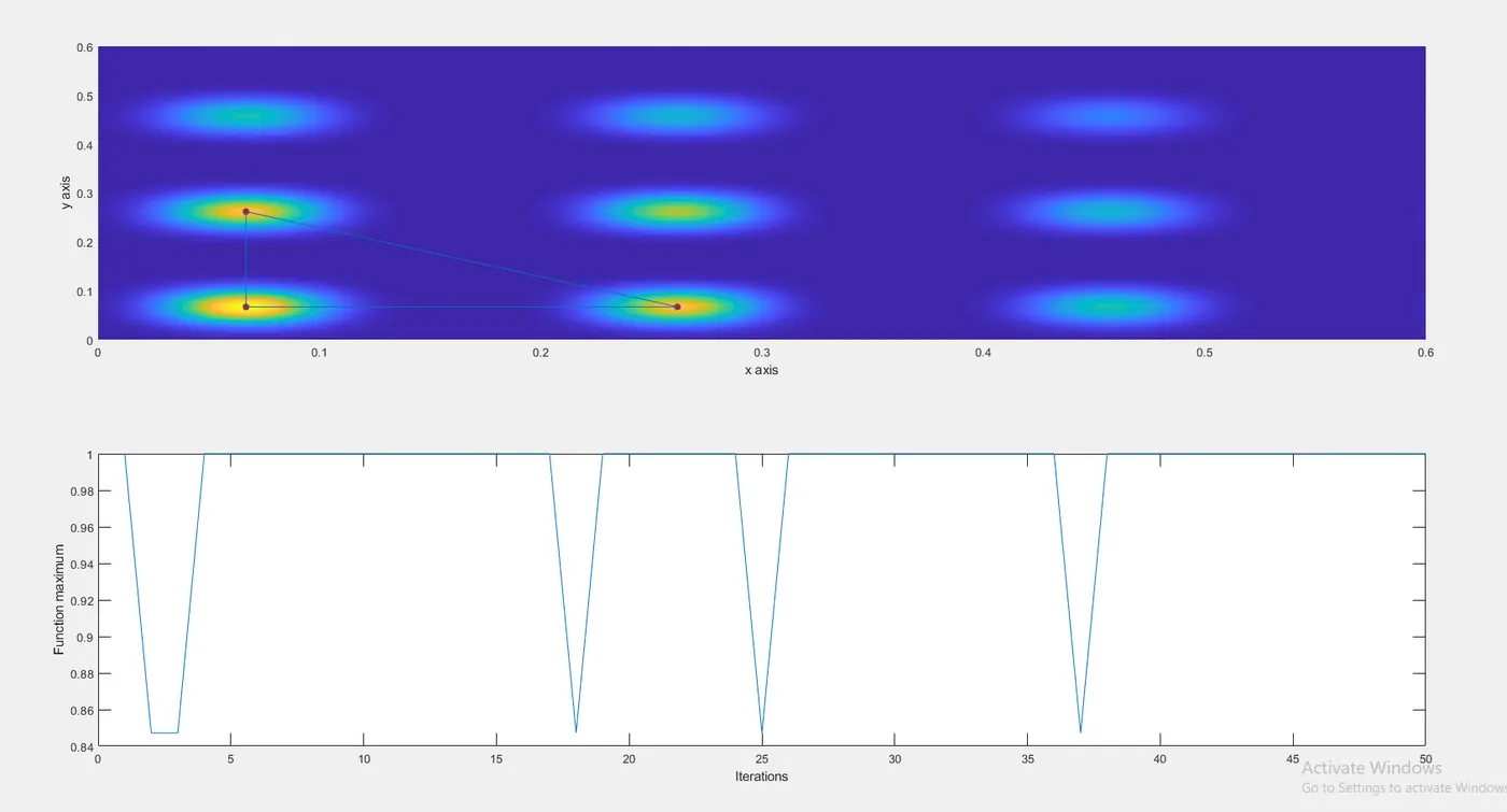
• Study - 2 showed that providing upper and lower limits can reduce the search space and thereby the offsprings produced were more similar to each other in each iteration.
• From the second subplot it was clear that there wasn't much variation in the optimum value of function maximum provided by the ga.
• This study showed that in order for the ga to arrive at a better offspring, the population size had to be increased.
• The time taken to run ga for study - 2 was 6.09 seconds.

Study - 3

Study - 3 is done to notice the change in result with an increase in population size.

It makes use of the ga syntax involving options.

The optimoptions command is used to change the optimization default values.

The population size default for ga is 50. We increase the population size and settle at one which provides results with less or no variation.

clear all
close all
clc

%inputs
x = linspace(0,0.6,150);
y = linspace(0,0.6,150);
number_cases = 50;

%Creating a 2D mesh for the x and y values
[xx yy] = meshgrid(x,y);

for i = 1:length(xx);
    for j = 1:length(yy);
        input_vector(1) = xx(i,j);
        input_vector(2) = yy(i,j);
        f(i,j) = stalagmite_func(input_vector);       
    end
end

% % Study 1 - Statistical behaviour of the genetic algorithm running this function. 
% tic
% for i = 1:number_cases
%     [inputs ,fopt(i)] = ga(@stalagmite_func,2);
%     xopt(i) = inputs(1);
%     yopt(i) = inputs(2);
% end
% Time_taken_study_1 = toc


% %Study 2 - Genetic algorithm search using upper and lower bounds
% tic
% for i = 1:number_cases
%     [inputs ,fopt(i)] = ga(@stalagmite_func,2,[],[],[],[],[0,0],[0.3,0.3]);
%     xopt(i) = inputs(1);
%     yopt(i) = inputs(2);
% end
% Time_taken_study_2 = toc


%Study 3 - Increasing the population to obtain optimum result
tic
options = optimoptions('ga','PopulationSize',180);
 for i = 1:number_cases
    [inputs ,fopt(i)] = ga(@stalagmite_func,2,[],[],[],[],[0;0],[0.5;0.5],[],options);
    xopt(i) = inputs(1);
    yopt(i) = inputs(2);
 end
 Time_taken_study_3 = toc

figure(2)
subplot(2,1,1)
surfc(xx,yy,-f)
hold on
shading interp
plot3(xopt, yopt,-fopt,'marker','o','markersize',5,'markerfacecolor','r')
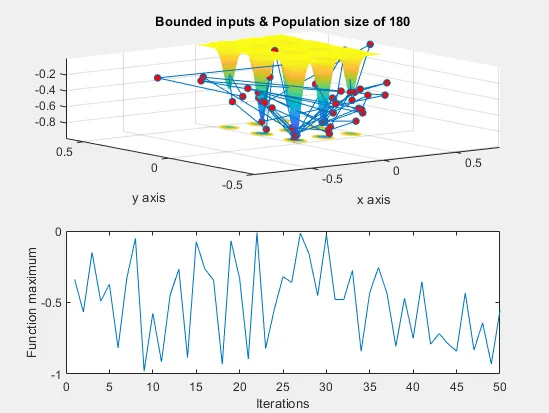
title('Bounded inputs & Population size of 180')
xlabel('x axis')
ylabel('y axis')
subplot(2,1,2)
plot (-fopt)
xlabel ('Iterations')
ylabel ('Function maximum')

Results of Study - 3

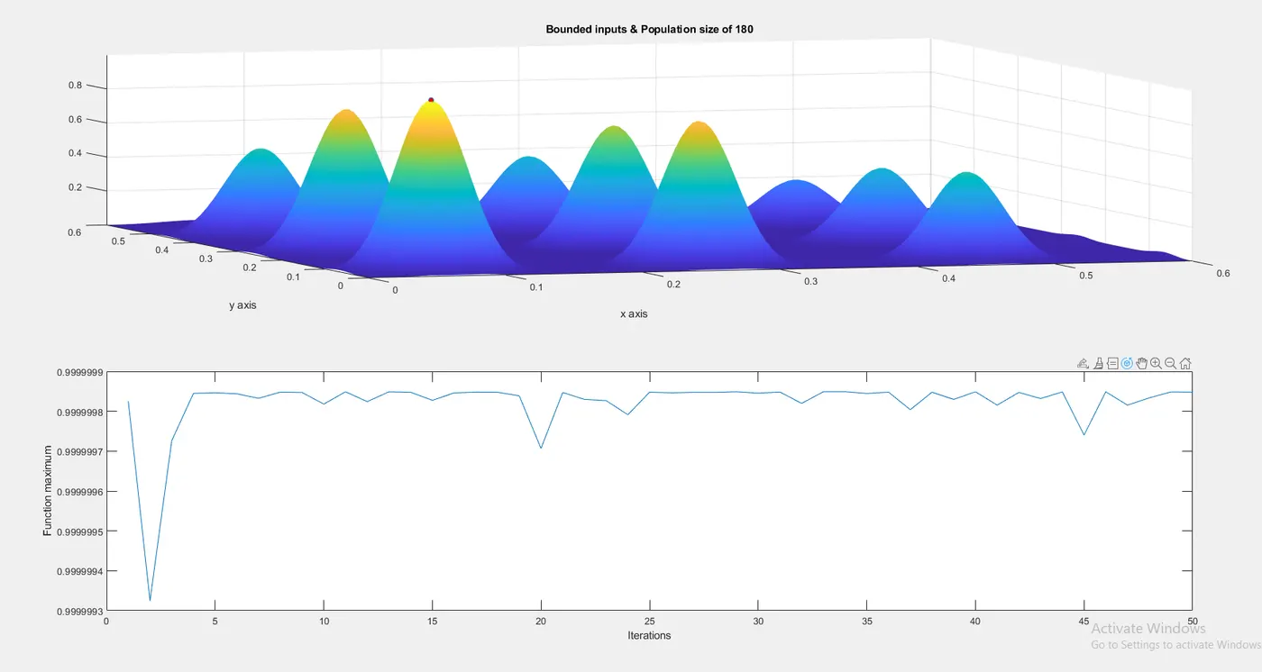
• The Study-3 provided with not much variation in the optimum value.
• The increase in population size resulted in an optimum value that was `~~`1 in all iterations as seen in the subplot.
• Increasing the population size causes the accuracy of ga to increase. We get more accurate results as the number of generations that converge increases.
• The time taken to run ga in the third study was 17.91 seconds.
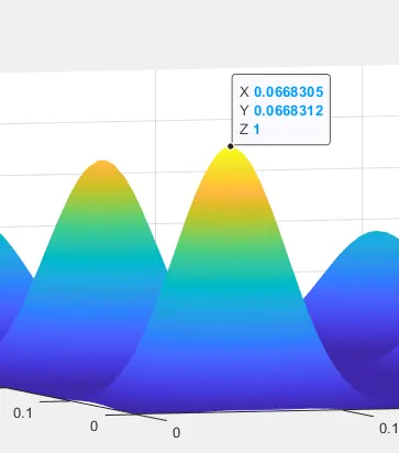
• The value for x and y at which the function reaches function maximum is given below.

Ending criteria

The ending criteria determines when a ga run has to stop. The following contains the ways by which the optimization gets terminated.

• When there is no improvement in population for a certain number of iterations.
• When the objective function has reached a certain pre-defined value.
• When we reach an absolute number of generations

Significance of running multiple iterations

Since the genetic algorithm uses randomness to select individuals, create initial offsprings, randomness in mutation and crossover methods and also randomness to slightly change individuals the results obtained may not be the same each time the ga is run.

In order to check if the ga gives the same optimum value every time it is run, we run multiple iterations in order to check if there's any variation in result.

Errors faced while Coding

The use of [] was not set for the inputs whose value was unknown. And it resulted in error.

Incorrect representation of function minima instead of maxima.

Several other spelling mistakes were made and had to be corrected.

Conclusion

The results for the three studies were plotted and the genetic algorithm was run to optimize the stalagmite function using MATLAB

References

https://www.tutorialspoint.com/genetic_algorithms/genetic_algorithms_introduction.htm

https://www.mathworks.com/help/gads/how-the-genetic-algorithm-works.html