Genetic Algorithm using Matlab

Finding the Global maxima of a function using the Genetic Algorithm via MATLAB.

Aim: The aim of the challenge is to solve a Global optimization problem by understanding the working of the Genetic Algorithm in Matlab and finding the Global maxima of a function.

Principle Theory:

Optimization is a procedure that is executed iteratively by comparing various solutions until an optimum or a satisfactory solution is found.

Optimization refers to finding the values of inputs in such a way that we get the “best” output values. The definition of “best” varies from problem to problem, but in mathematical terms, it refers to maximizing or minimizing one or more objective functions, by varying the input parameters.

As explained above we need to choose an optimization algorithm to perform the Optimisation process. Genetic Algorithm is one of the optimization processes.

Genetic algorithms are commonly used to generate high-quality solutions to optimization and search problems by relying on biologically inspired operators such as mutation, crossover, and selection. The genetic Algorithm in Matlab always minimizes the function.

There are five important features of GA:

Fitness Function represents the main requirements of the desired solution of a problem (i.e. cheapest price, shortest route, most compact arrangement, etc). This function calculates and returns the fitness of an individual solution. The Fitness function used here is the Stalagmite function.

The Stalagmite Function in this model will help us to generate local minima and maxima.

Encoding possible solutions to a problem are considered as individuals in a population. If the solutions can be divided into a series of small steps (building blocks), then these steps are represented by genes and a series
of genes (a chromosome) will encode the whole solution. This way different solutions to a problem are represented in GA as chromosomes of individuals.

The selection defines the way individuals in the current population are selected for reproduction. There are many strategies for that (e.g. roulette–wheel, ranked, tournament selection, etc), but usually the
individuals which are more fit are selected.

The crossover operator defines how chromosomes of parents are mixed in order to obtain genetic codes of their offspring. This implements the inheritance property (offspring inherit genes of their parents).

The mutation creates random changes in the genetic codes of the offspring. This is needed to bring some random diversity into the genetic code. In some cases, GA cannot find the optimal solution without a mutation operator (local maximum problem).

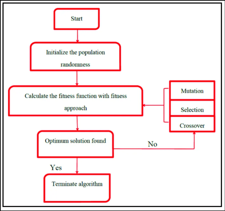
The following chart shows how the Genetic Algorithm works to find the optimum solution.

Matlab Code:

Case Study 1:

In case study 1 we will be just be applying the Genetic Algorithm and see how the program performs without any constraints.

clear all
close all
clc

x=linspace(0,0.6,150);
y=linspace(0,0.6,150);
num_cases=50
[xx, yy]=meshgrid(x, y);

So in the beginning we are providing the x and y inputs using the linspace command and the Num_Cases which is the iteration number. Since x and y are both a One-Dimensional array we are using the Mesh grid to form a Two-dimensional array represented by xx and yy.

for i=1:length(xx)
    for j=1:length(yy)
        input_vector(1)=xx(i,j);
        input_vector(2)=yy(i,j);
        F(i,j)=stalagmite(input_vector);
      end 
end

This For loop will run for the length of the xx and yy, The input function is a row vector with two columns which we are assigning using Input_vectoe(1) and (2).

The Stalagmite function here will help us in finding the local maxima and minima. This loop is used entirely for the plotting of the 3-D Graph so that we can easily understand the working. The Stalagmite function is a function that we call into this Program.

The Formula for the Stalagmite function is below.

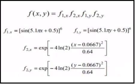
The two variables in the function are x and y. We need to convert this formula into Matlab code so that we can call it in.

function[F]=stalagmite(input_vector)
x=input_vector(1);
y=input_vector(2);
f1=(sin(5.1*pi*x+0.5))^6;
f2=(sin(5.1*pi*y+0.5))^6;
f3=exp(-4*log(2)*((x-0.0667)^2/0.64));
f4=exp(-4*log(2)*((y-0.0667)^2/0.64));
F=f1*f2*f3*f4*-1;
end

We can see that F will be the output for the above function and, Input_vector(1) and Input_vector(2) being x and y. Then we code the formula as it is so that we find the value of F.

We already know that Ga will only find the Global minima (i.e) using the Stalagmite function it can only find the lowest value. So we need to make a small change in the final step of the function so that Ga will be able to find the Global maxima so we will be introducing a"-" sign to F so that Ga can find the Global maxima.

%Study 1- Statistical behaviour
tic
for i=1:num_cases
    [inputs, fopt(i)]=ga(@stalagmite,2);
    xopt(i)=inputs(1);
    yopt(i)=inputs(2);
end

study1_time=toc

For the first case study, we will be running the Ga algorithm without any bounds Lower bound or Upper bound and the default population 50. And since Ga is an iterative solver the loop is fun for 50 loops.

The inputs have two values the x and y coordinate of the fopt. we can see that the stalagmite function is used and the variable two are inputted. The xopt is the "x" value from the input and yopt is the "y" value. And we will be calculating the time taken using the tic and toc commands

Syntax of Genetic Algorithm in Matlab:

x=ga(@fun,nvars,A,B,Aeq,Beq,Lb,Ub,nonlcon,intcon,options)

• fun= The fitness function in our case the Stalagmite function.
• nvars= number of variables (2)
• A and B= Linear inequalities of the Form A*x<=B
• Aeq and Beq=Linear equalities of the form A*x=B
• LB and UB=Lower and Upper bound that is the region in which Ga will search for the result.
• nonlcon=non Linear inequalities
• intcon=Integer constrained
• options= Helps to add constrain tolerance by increasing the population size.
• For our first case, all the above options are not used so Ga will assume the default values.

subplot(2,1,1)
surfc(xx,yy,-F)
hold on
shading interp
plot3(xopt,yopt,-fopt,'marker','o','markersize',5,'markerfacecolor','r')
title('Unbounded inputs')
xlabel('X-axis')
ylabel('Y-axis')
subplot(2,1,2)
plot(fopt)
xlabel('Iterations')
ylabel('Function Maxima')

We will be creating two plots so we will be applying the subplot command. The surfc is used to view the 3-D graph of the points xx,yy,-F, Here the -F is to represent the graph in the positive axis. Hold on is used to views all the plots. Sharp interp is used so that the 3-D graph is more representable.

Plot 3 is used to plot all the three values xopt,yopt and -fopt in the 3-Graph and the second Subplot only views the fopt in a 2-D graph.

Graph:

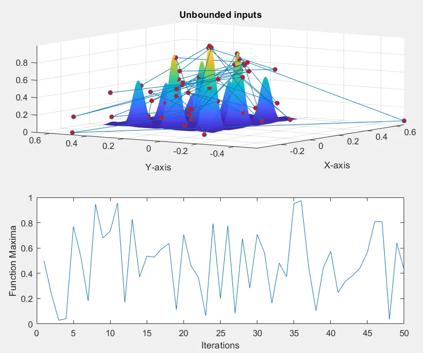
The Red points represent the Maxima value that the function is trying to predict in 50 iterations. You can see that it is searching over a range of areas in the x-axis and y-axis as we have not given the upper and lower bounds.

In the second graph, you can see that the Fopt value range from 0 to 1 but with various peaks hence this method is not enough to find the maximum value. In this case, we are not able to find the Global maxima as the Algorithm is not able to predict it correctly.

The time is taken for this study to run is 2.9042s

Case Study-2

Since we are able to see the Surface graph from the first study we can assume where the Maximum will be hence so we will be directing the algorithm to search in that region.

%Study-2(Statistical behavior-With Upper and Lower bounds)
tic
for i=1:num_cases
    [inputs, fopt(i)]=ga(@stalagmite,2,[],[],[],[],[0;0],[0.5;0.5]);
    xopt(i)=inputs(1);
    yopt(i)=inputs(2);
end
study2_time=toc

Only this region of the code will be modified in the second case study. You can see that we are giving the upper and lower bounds value (0,0) and (.5,.5). We are instructing the algorithm that the maximum will be under that region. The Population for this study will be 50 which is the default value.

Graph:

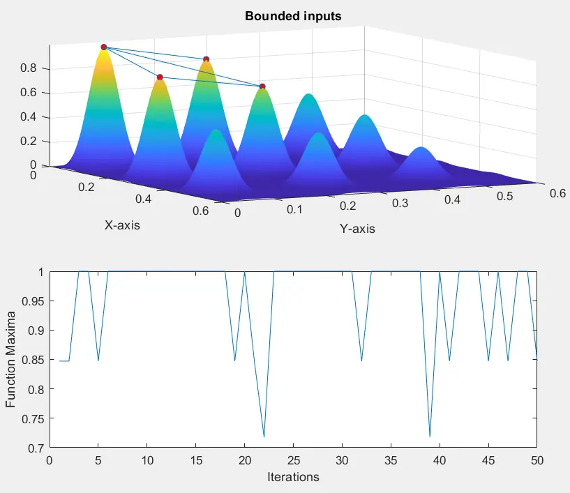
You can see that after we applied the Lower and Upper bound the results are much better. The Algorithm has reduced down the Global maxima between 4 points. This is because we have reduced the search space. This result is okay considered to the previous result but we need to find only the single global maxima.

You can also see from the second graph that the Maximum value range is from 0.5 to 1. The Time taken for this run is 4.0093 which has increased from the first case study.

The Entire code for Case Study two is below:

clear all
close all
clc

x=linspace(0,0.6,150)
y=linspace(0,0.6,150)
num_cases=50
[xx, yy]=meshgrid(x, y);

for i=1:length(xx)
    for j=1:length(yy)
        input_vector(1)=xx(i,j);
        input_vector(2)=yy(i,j);
        F(i,j)=stalagmite(input_vector);
      end 
end

%Study-2(Statistical behavior-With Upper and Lower bounds)
tic
for i=1:num_cases
    [inputs, fopt(i)]=ga(@stalagmite,2,[],[],[],[],[0;0],[0.5;0.5]);
    xopt(i)=inputs(1);
    yopt(i)=inputs(2);
end
study2_time=toc

subplot(2,1,1)
surfc(xx,yy,-F)
hold on
shading interp
plot3(xopt,yopt,-fopt,'marker','o','markersize',5,'markerfacecolor','r')
title('Bounded inputs')
xlabel('X-axis')
ylabel('Y-axis')
subplot(2,1,2)
plot(-fopt)
xlabel('Iterations')
ylabel('Function Maxima')

Case Study-3

In this case study, we will be increasing the population number from 50 which is the default value a to 250. The higher the number of the population it increases the probability of us finding the optimum function.

There are several things to be kept in mind when dealing with GA population −

• The diversity of the population should be maintained otherwise it might lead to premature convergence.

• The population size should not be kept very large as it can cause a GA to slow down, while a smaller population might not be enough for a good mating pool. Therefore, an optimal population size needs to be decided by trial and error.

So in this case the Population is 250 and the other values are the same as of the second case study. So the time taken to run the program will be more for this case.

%Study 3 Incresing the GA Iteration
options=optimoptions('ga');
options=optimoptions(options,'PopulationSize',250);

tic
for i=1:num_cases
    [inputs, fopt(i)]=ga(@stalagmite,2,[],[],[],[],[0;0],[0.5;0.5],[],[],options);
    xopt(i)=inputs(1);
    yopt(i)=inputs(2);
end
study3_time=toc

You can see from that the options command is used to provide the value of the population. The optimoptions command is used to create the optimization options for the Ga algorithm and the population size is inputted.

Graph

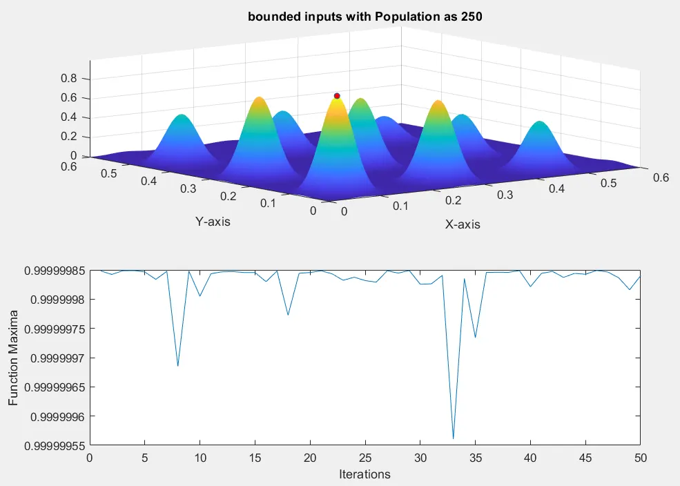
You can see from the above graph that Ga has found our Global Maxima. So after we increased the population size and provided the upper and lower bound the algorithm was able to find the value by itself. The time has increased to 14.576s for this run.

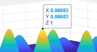
You can see that the Maximum value is in the above image.

Complete code for the 3rd Case Study:

clear all
close all
clc

x=linspace(0,0.6,150)
y=linspace(0,0.6,150)
num_cases=50
[xx, yy]=meshgrid(x, y);

for i=1:length(xx)
    for j=1:length(yy)
        input_vector(1)=xx(i,j);
        input_vector(2)=yy(i,j);
        F(i,j)=stalagmite(input_vector);
      end 
end

%Study 3 Incresing the GA Iteration
options=optimoptions('ga');
options=optimoptions(options,'PopulationSize',250);

tic
for i=1:num_cases
    [inputs, fopt(i)]=ga(@stalagmite,2,[],[],[],[],[0;0],[0.5;0.5],[],[],options);
    xopt(i)=inputs(1);
    yopt(i)=inputs(2);
end
study3_time=toc

subplot(2,1,1)
surfc(xx,yy,-F)
hold on
shading interp
plot3(xopt,yopt,-fopt,'marker','o','markersize',5,'markerfacecolor','r')
title('bounded inputs with Population as 250')
xlabel('X-axis')
ylabel('Y-axis')
subplot(2,1,2)
plot(-fopt)
xlabel('Iterations')
ylabel('Function Maxima')

Errors Faced:

Errors faced due to spelling mistakes which were corrected.

The plotting on the other direction as missed to five the minus sign in "plot3(xopt,yopt,fopt,'marker','o','markersize',5,'markerfacecolor','r')" which was rectified to -fopt.

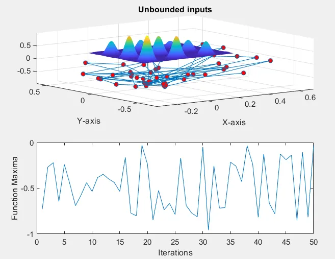
Wrongly entered the xopt(i) to 1 and yopt(i) to 1 which lead to the below error. Which was later corrected.

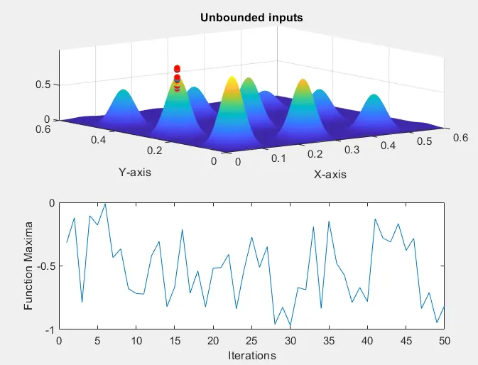
Conclusion:

In this challenge, the concept of a Genetic algorithm was used to optimize the stalagmite function to find the Global maxima. The concept and working of genetic algorithm are studied and used in the three cases to optimize the function and find the Global maxima.