Mixing efficiency
Problem Definition
We have to set up steady-state simulations to compare the mixing effectiveness when the hot inlet temperature is 360C & the Cold inlet is at 190C for short and long mixing tee.
We have to use the k-epsilon and k-omega SST models for the first case and based on the result we have to use the more suitable model for further cases.
The inlet velocity of hot air is 3 m/s. For the momentum ratio of 2 and 4, we have to solve the problem for both long and short mixing tee.
Introduction
The ratio of the cold air velocity to the hot air velocity is the momentum ratio of the mixing tee.

We calculate the analytical value of the temperature at the outlet of the pipe by this formula

where
T = Temperature of the fluid
m = mass flow rate of the fluid = `rho*A*V`
where:- `rho`= Density of the fluid
A = Cross-section area of the pipe = 8.9*`10^-4`
V = velocity of the fluid
So for momentum ratio of 2
`T_(mixture)` = `(rho*8.9*10^-4*3*36+rho*8.9*10^-4*6*19)/(rho*8.9*10^-4*3+rho*8.9*10^-4*6)`= 24.6
So for momentum ratio of 4
`T_(mixture)` = `(rho*8.9*10^-4*3*36+rho*8.9*10^-4*12*19)/(rho*8.9*10^-4*3+rho*8.9*10^-4*12)`= 22.4
Mixing Tee
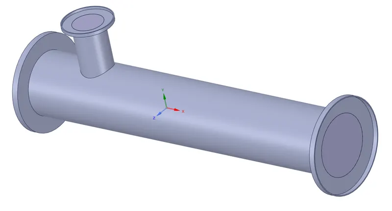
Mixing Tees utilizes a specifically engineered internal geometry to efficiently mix two fluid streams into one combined stream. It is useful in the air conditioning system and hot water system.
We are going to check that what happens when we increase the length of the pipe and what happens when we increase the inlet velocity of the cold air.
Turbulence
In fluid dynamics, turbulence or turbulent flow is fluid motion characterized by chaotic changes in pressure and flow velocity. It is in contrast to a laminar flow, which occurs when a fluid flows in parallel layers, with no disruption between those layers.
Turbulence is commonly observed in everyday phenomena such as surf, fast-flowing rivers, billowing storm clouds, or smoke from a chimney, and most fluid flows occurring in nature or created in engineering applications are turbulent. Turbulence is caused by excessive kinetic energy in parts of a fluid flow, which overcomes the damping effect of the fluid's viscosity. For this reason turbulence is commonly realized in low viscosity fluids.
Turbulence is an irregular motion of the air resulting from eddies and vertical currents. It may be as insignificant as a few annoying bumps or severe enough to momentarily throw an airplane out of control or to cause structural damage. Turbulence is associated with fronts, wind shear, thunderstorms, etc.
The onset of turbulence can be predicted by the dimensionless Reynolds Number, the ratio of kinetic energy to viscous damping in a fluid flow. The flow said to be turbulent flow when the Reynolds number is higher than 2300 the flow is said to be turbulent flow.
Convergence
As most of the fluid flow problems are non-linear in nature, dealing with inherently unstable phenomena such as turbulence. The solution techniques use an iterative process to successively improve a solution until ‘convergence’ is reached.
When the simulation has no change on all the convergence criteria, after certain iterations or timesteps, then we can consider that the solution has reached a steady-state, i.e.., converged. Even if we run further long, we will not be able to see any changes.
The following criteria's need to be monitored as the analysis progresses
(i) Residual value- No changes after some iteration and follows the same pattern
(ii) Solution imbalances
(iii) By observing the quantity of interest- No changes after some iteration
Y+
The y+ value is a non-dimensional term that can be used to understand how coarse or fine our grid is. This can then be used to determine if wall functions need to be used or not.
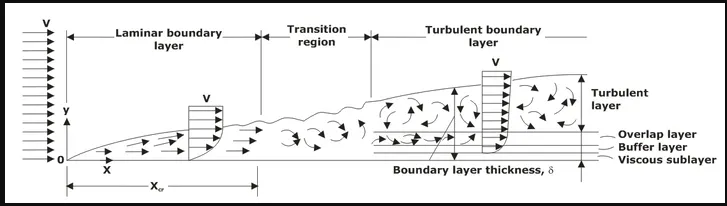
When the fluid is the flow above the flat plate and we have the turbulent flow of the fluid. In this case initially the fluid is laminar after some time it goes to the transition flow and eventually in the end it becomes turbulent. So when the flow is in the turbulent boundary layer. There are two boundary in there. The first boundary is viscosity dominant and the second boundary is inertia forces dominant.
In the first boundary there are three layers first is the viscous sublayer where the flow is laminar, second layer is buffer layer where the flow is transient and in the third layer (overlap layer) flow is turbulence.
If we are taking our first cell in the viscous sublayer then our Y+ value should be less than 5, when the first cell in the buffer layer the Y+ value lies between 5 to 30 and when it is in the overlap layer the Y+ value should be more than 30. When we have the Y+ value more than 30 solver is going to use wall function.

where
y = distance from the wall
`u_t`= frictional velocity
`nu`= kinematic viscosity
K-`epsilon` model
K-epsilon (k-ε) turbulence model is the most common model used in CFD to simulate mean flow characteristics for turbulent flow conditions. It is a two-equation model that gives a general description of turbulence by means of two transport equations (PDEs).
(i) The first transported variable is the turbulent kinetic energy (k).
(ii) The second transported variable is the rate of dissipation of turbulent kinetic energy (ε).
We use the K-`epsilon` model when the Y+ value is more than 30. So the first cell should be in the overlap layer. It is used for the high Reynolds number.
The realizable k-ɛ model differs from the standard k−ɛ model in two ways. Firstly that in the realizable k-`epsilon` model the kinematic viscosity is not constant like in the standard model but a variable. The second difference is a new transport equation for the dissipation rate, ɛ, that is derived from an exact equation for the transport of the mean-square vorticity fluctuation.
K-`omega` model
In CFD, the k–omega (k–ω) turbulence model is a common two-equation turbulence model, that is used as an approximation for the RANS equations. The model attempts to predict turbulence by two partial differential equations for two variables, k and ω, with the first variable being the turbulence kinetic energy(k) while the second (ω) is the specific rate of dissipation (of the turbulence kinetic energy k into internal thermal energy).
The standard k−ω model is a low Re model, i.e., it can be used for flows with low Reynolds number where the boundary layer is relatively thick and the viscous sublayer can be resolved.
We use the K-`omega` model when the Y+ value is less than 5. So our first cell should be in the viscous sublayer.
SST stands for shear stress transport. The SST formulation switches to a K-`epsilon` behavior in the free-stream, which avoids the k−ω problem of being sensitive to the inlet free-stream turbulence properties.
The k−ω SST model provides a better prediction of flow separation than most RANS models and also accounts for its good behavior in adverse pressure gradients.
Case Setup
1. First we are going to open the workbench and going to click on the Fluid Flow(Fluent). It is going to open the module in the Project Schematic.
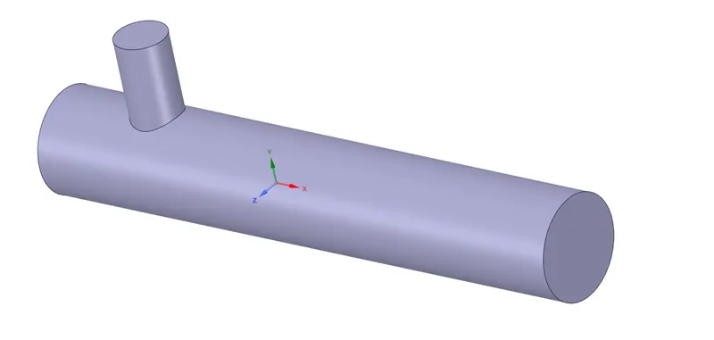
2. Now we are going to click on the geometry. It will take you to the spaceClaim. Here we are going to open the existing design. So now we can see the original design. On which we are going to do our simulation. When we open the original file it opens the solid model but we are not going to do the solid simulation. We are just going to do the fluid simulation so we are going to just extract the fluid volume.
3. To extract the fluid volume first, we are going to click on the 'Prepare'. There is an option 'Volume Extract'. In that, we can see an option of 'Edge Extract'. So now we are going to select the edges which we have required and going to click on the right sign. Now we are going to name the inlet, outlet, and wall to the design.
4. Now we are going to uncheck the box of the solid and we are going to suppress it for further calculation. Our geometry is prepared. Now we are going to close the spaceClaim.
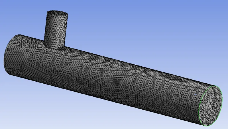
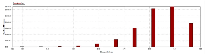
5. Now we are going to click on the mesh. It will take us into the meshing. Here we decide what mesh element size we are going to take and we are going to check that the quality of the mesh. If the mesh quality is greater than 5 it is a good mesh. Now we are going to name the inlet, outlet, and wall to the design. So our meshing is done.
mesh
Quality
6. Now we are going to update the mesh. Now we are going to Setup the case. So it will take us to the Fluent. So we are solving the 3-D problem. We are going to use double precision and we are going to use 4 Solver Processes(parallel). So now when we start it will take us to the Fluent.
7. In the Fluent we will go to Physics. Here we choose the type of solver, we have taken the pressure-based type solver. Now we have to choose the velocity formulation, we have taken absolute velocity formulation. Now we are going to choose the time, we are using a steady time. We have to calculate the temperature so we are going to use the energy equation also.
8. Now we are going to choose which type of model we are considering. In this case, we are using k-`epsilon` and k-`omega`.
9. Now we are going to give the boundary conditions. The velocity and temperature to the hot and cold air. Other than that we are going to use the default boundary conditions.
10. Now we are going to click on the solution. Here we are going to create the definitions, First, we are going to select the type of the report, Then the field variable, now we are going to choose the surface at which we want the result. We are going to check the plot and report both boxes.
11. We can give the residual criteria. Now we are going to initialize the values and we are going to give the iteration number for which we want the simulation. Now we are going to calculate the result.
12. After the completion of the simulation it shows us the plots we have defined in the definitions and we get all the results. So our result has been calculated.
13. Now we are going to update our results. So when we click on the results it takes us to the CFD-post processing. Here we can see what effects (temperature and velocity) are occurring when we mix hot and cold air. We are going to plot the effect of the temperature and velocity in the pipe along the pipe length and across the pipe cross-section.
15. On the basis of those results we are going to make our conclusion.
Case-1
Short length pipe with momentum ratio of 2 using k-`epsilon` model
So in this case we have taken the element size = 0.002 m
We are going to use realizable k-ɛ model
For hot air
Inlet temperature = 36 degree celcius
Inlet velocity = 3 m/s
For cold air
Inlet temperature = 19 degree celcius
Inlet velocity = 6 m/s
Solution
Residual
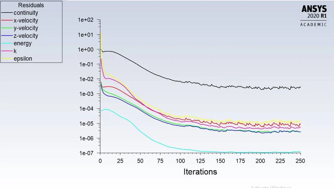
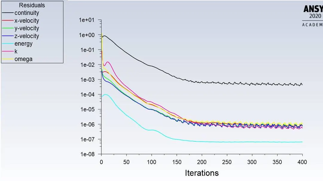
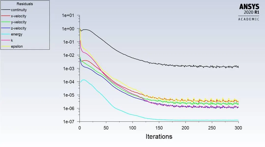
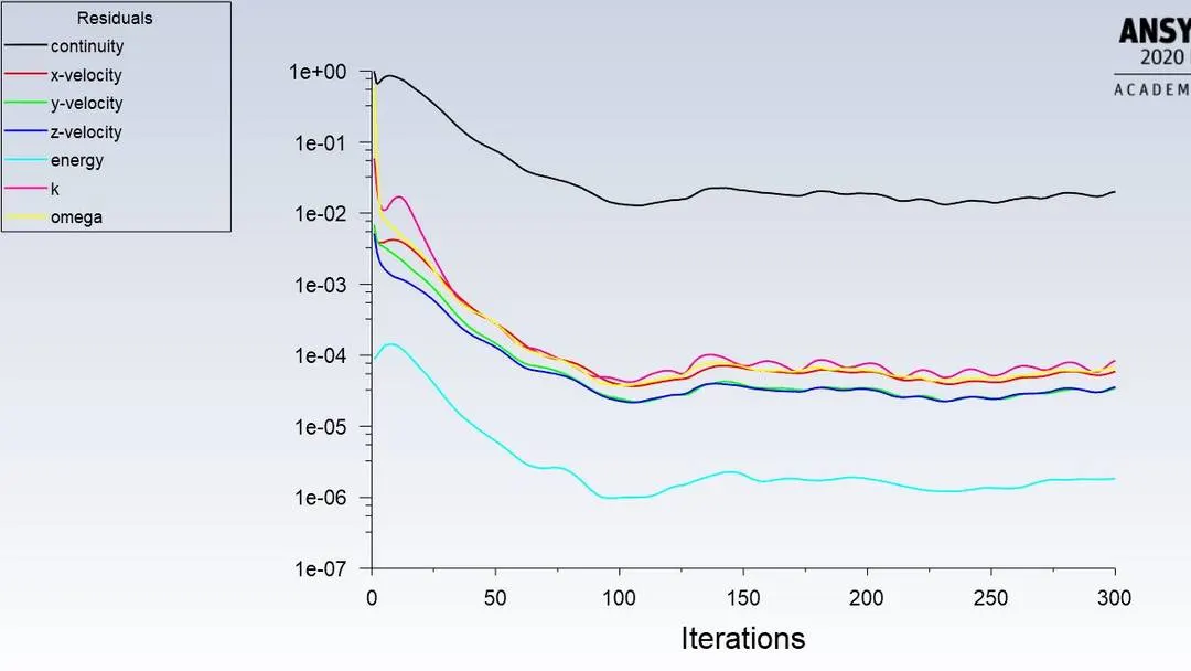
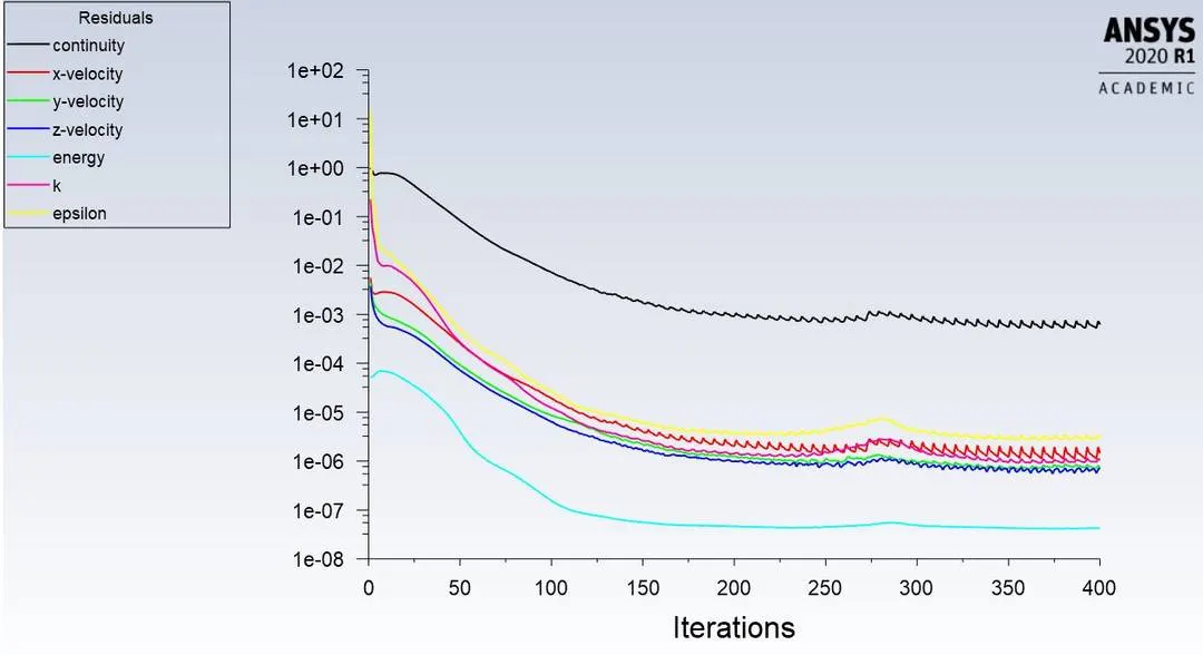
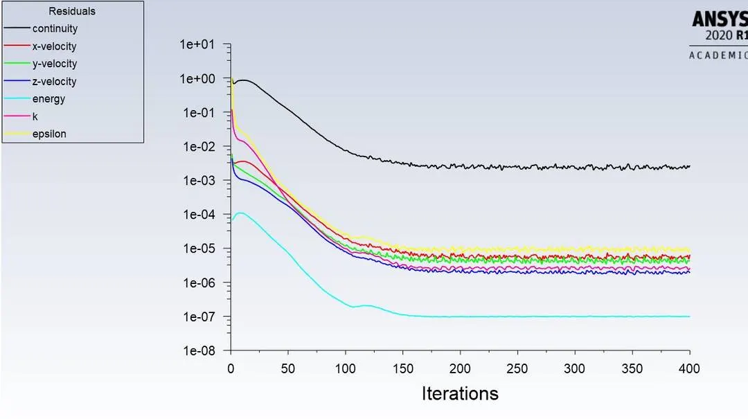
We can see from the residual graph that after some iteration the values did not change so we get the convergence results.
Temperature
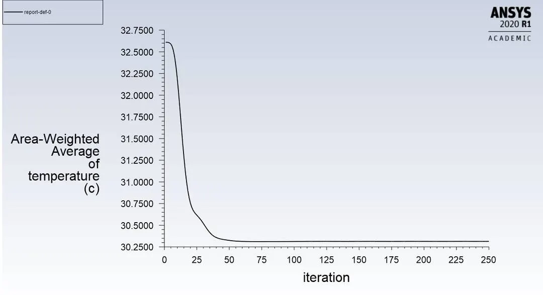
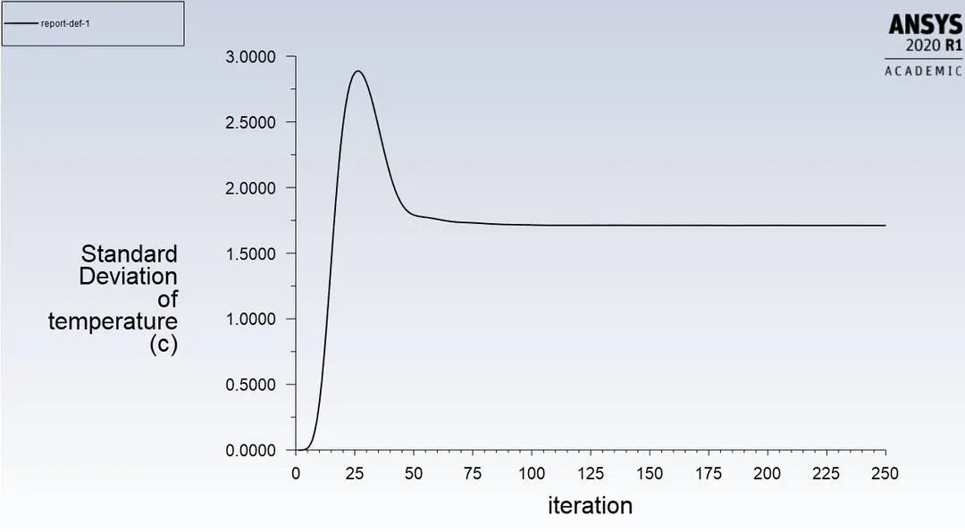
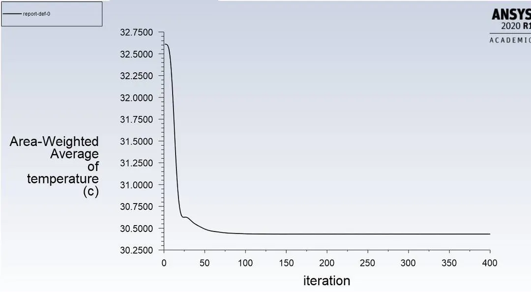
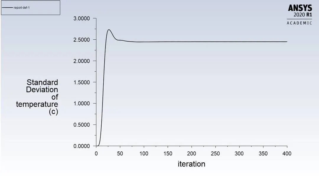
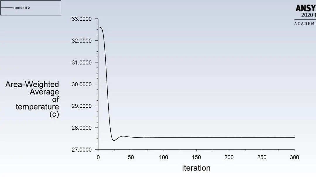
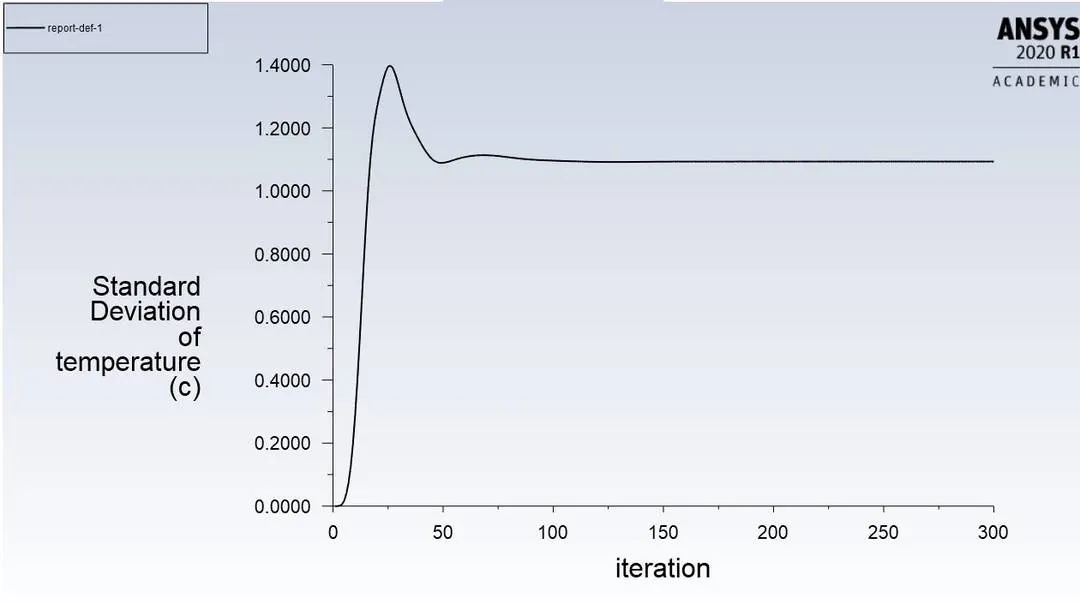
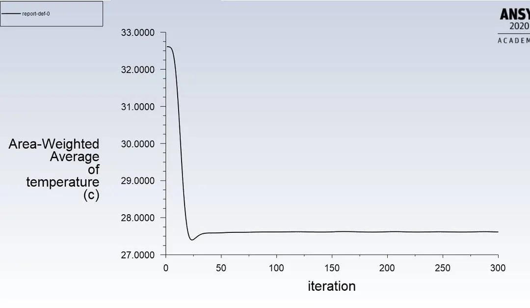
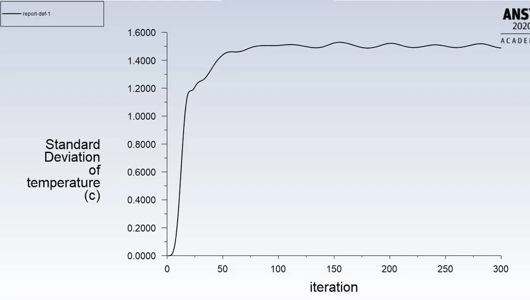
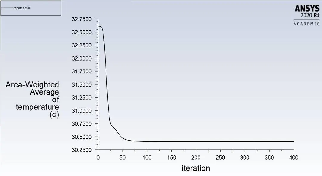
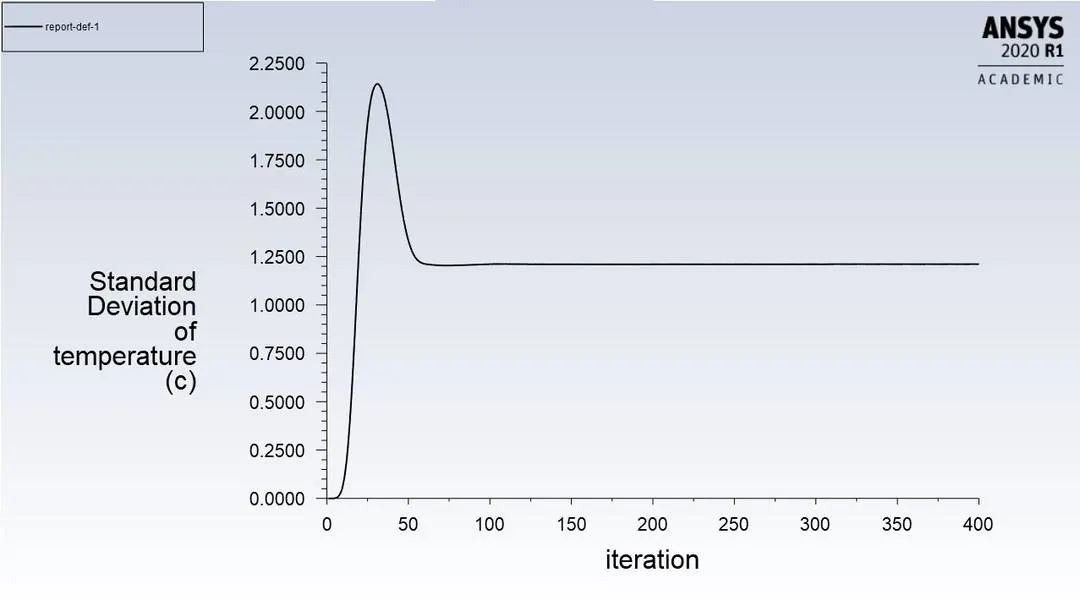
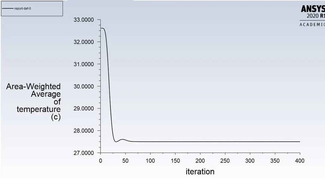
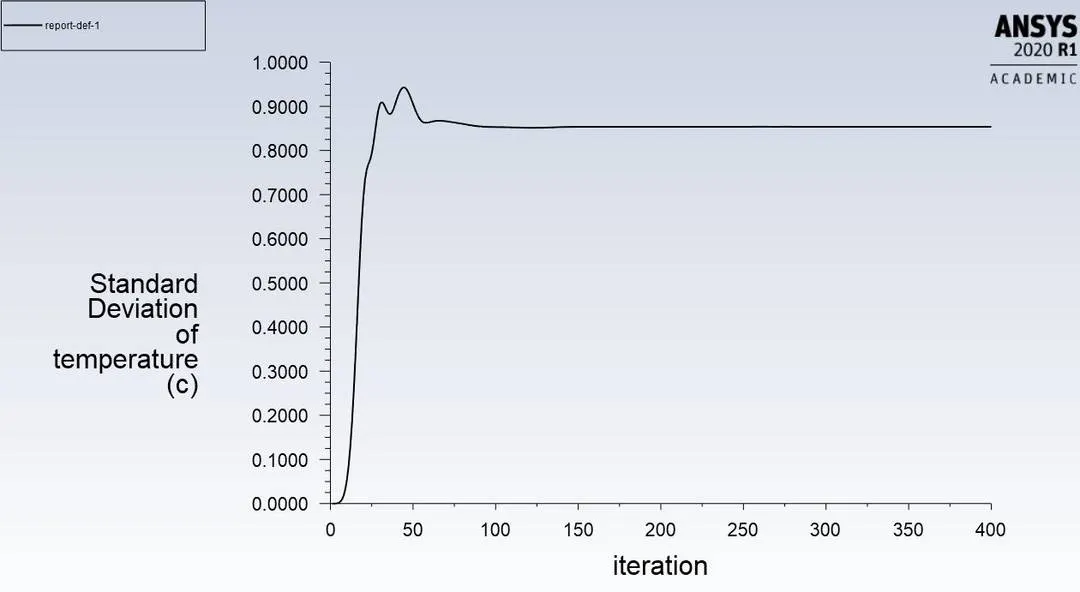
Area-Weighted Average of temperature graph is showing us how the average temperature value is changing with each iteration at the outlet and Standard Deviation of temperature is showing that how the efficiency of the mixing of the hot and cold air are changing with each iteration at the outlet.
So because our result got convergence so after some iteration our average temperature value and standard deviation are not going to change.
Velocity
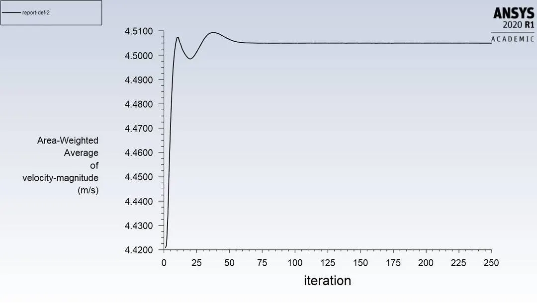
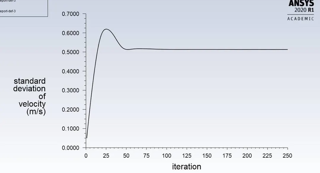
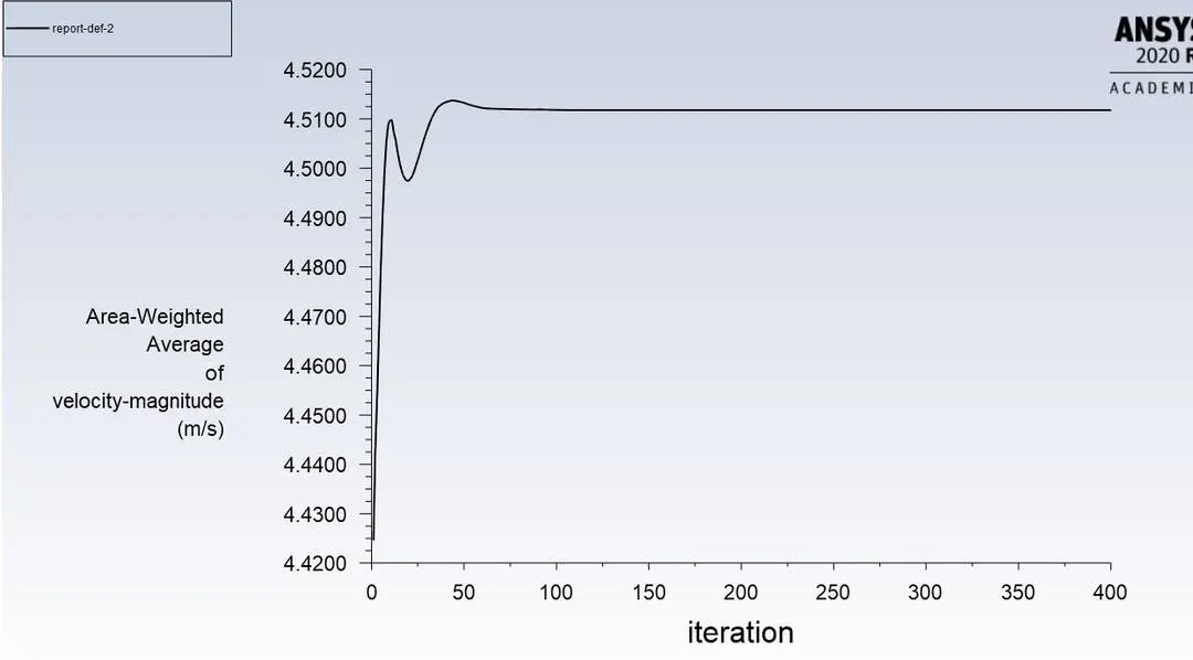
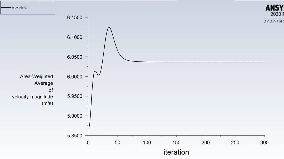
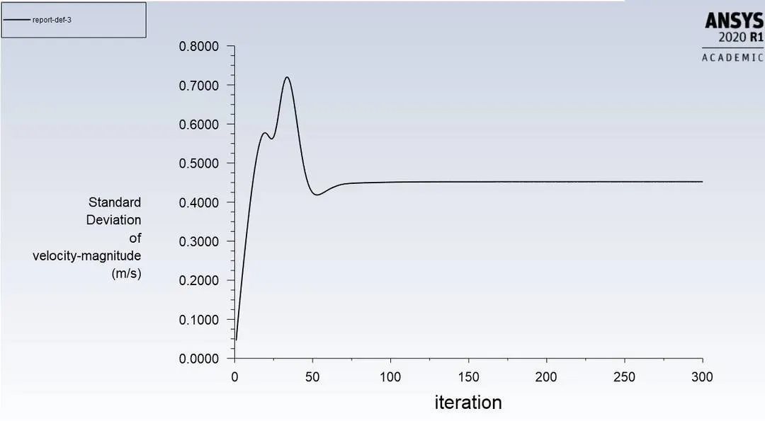
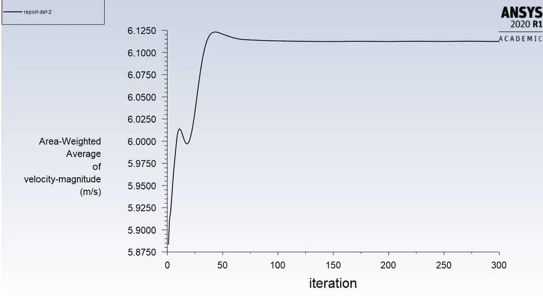
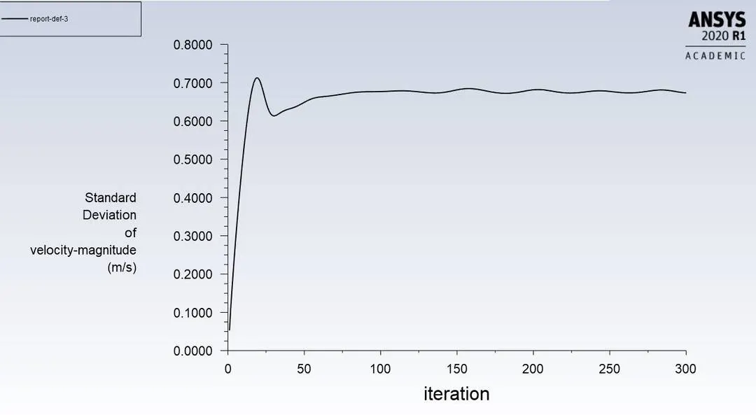
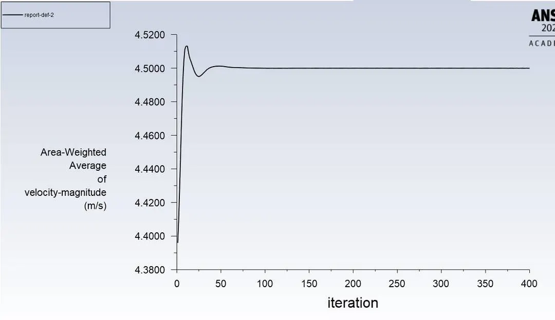
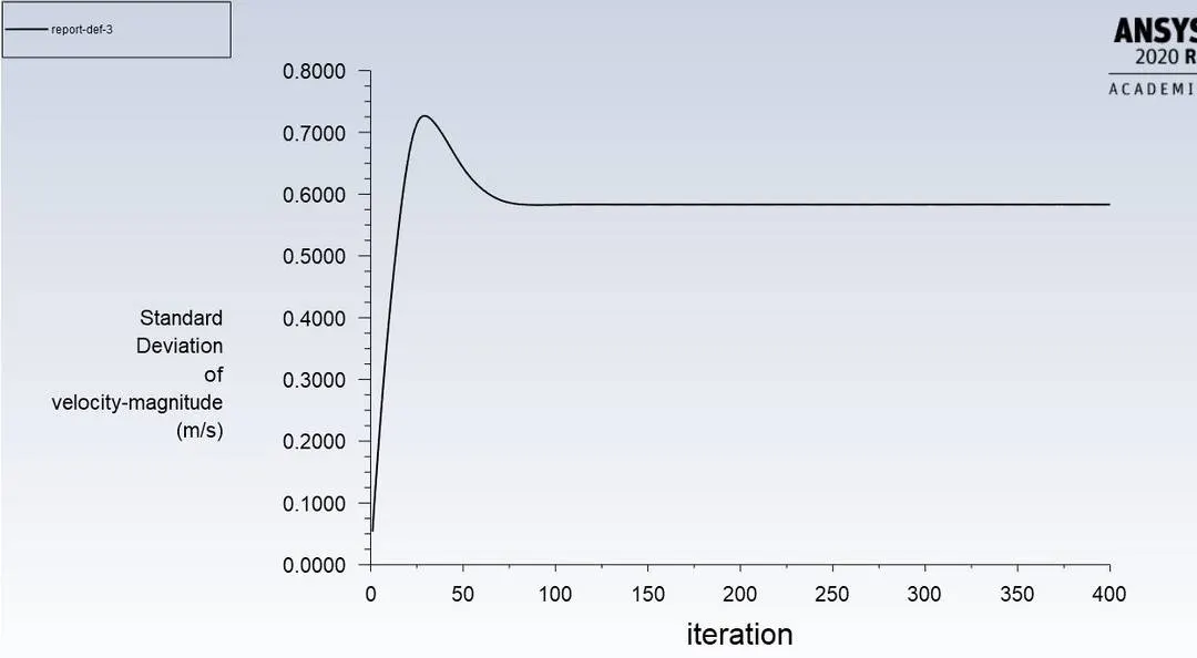
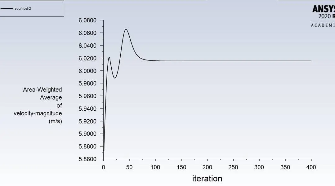
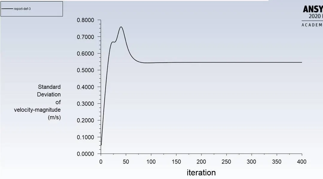
Area-Weighted Average of velocity graph is showing us how the average velocity value is changing with each iteration at the outlet and Standard Deviation of velocity is showing that how the efficiency of the mixing of the hot and cold air are changing with each iteration at the outlet.
So because our result got convergence so after some iteration our average velocity value and standard deviation are not going to change.
Result
Post Processing
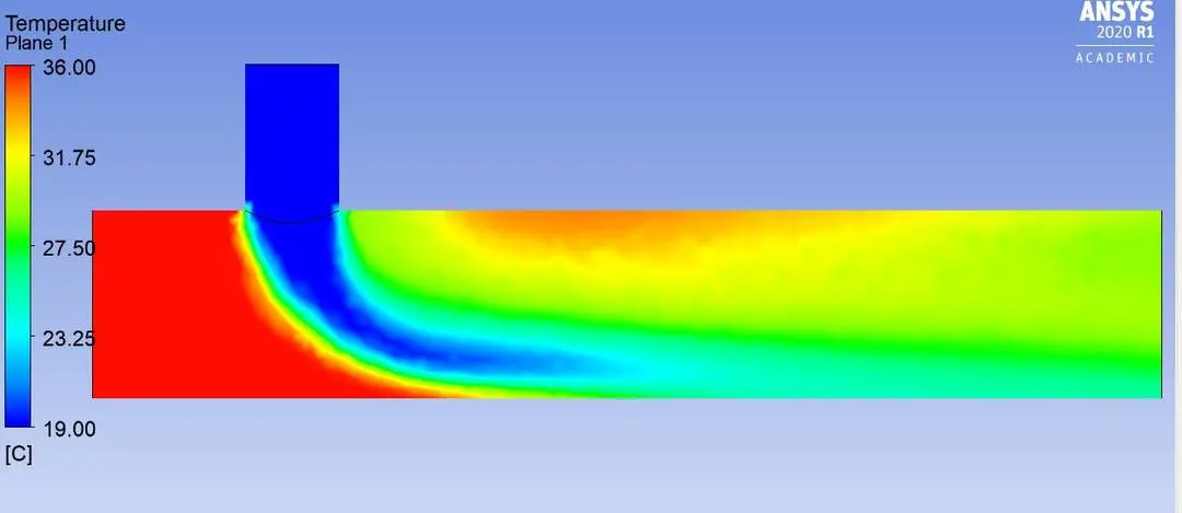
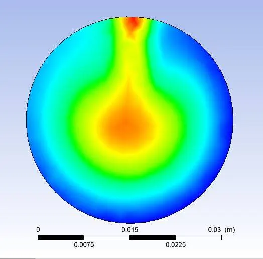
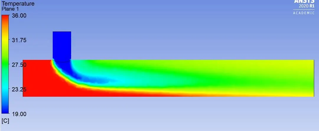
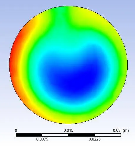
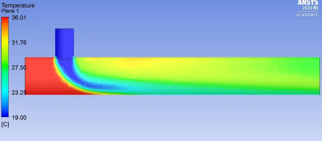
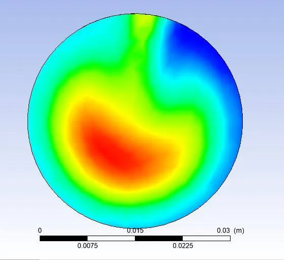
Effects of the temperature on the pipe across it's length and at the outlet
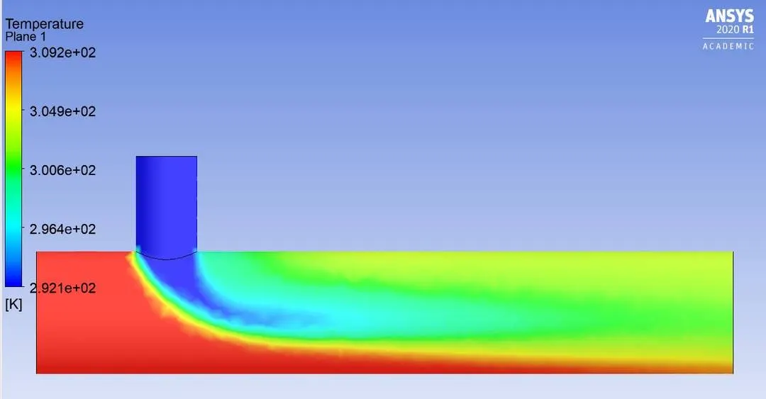
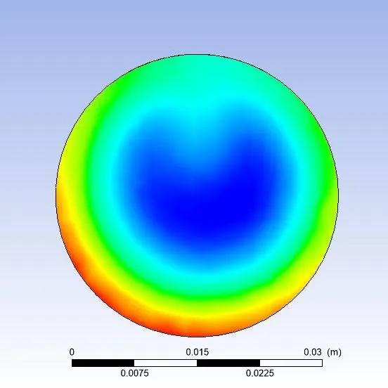
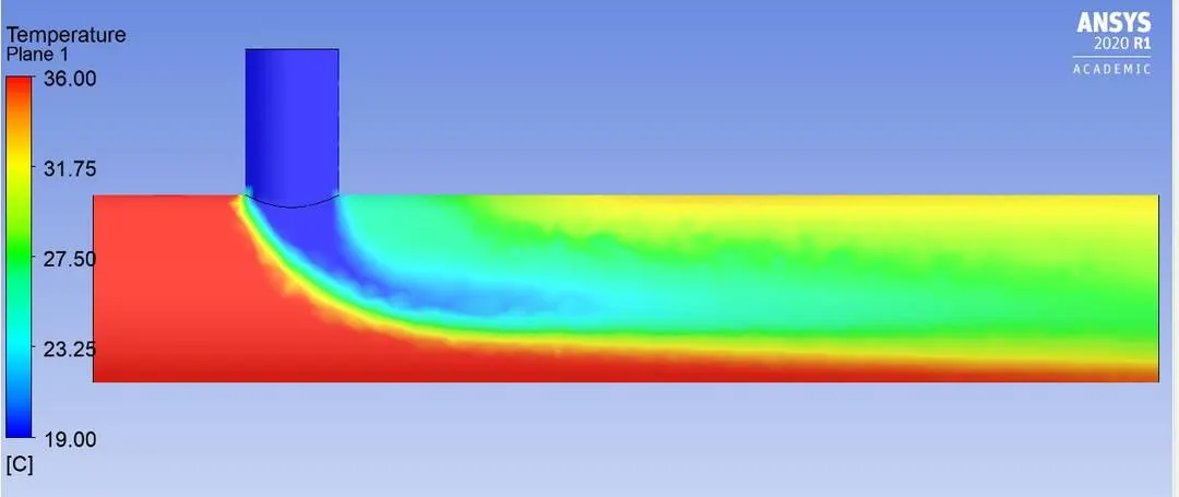
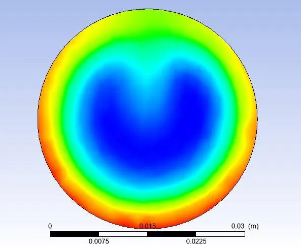
So in the above pictures, we can say that the temperature is different at every point in the mixing tee and in the outlet the temperature is minimum at the mid of the pipe and the temperature is maximum at the boundary of the pipe it is maximum.
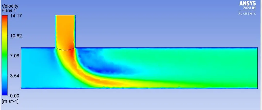
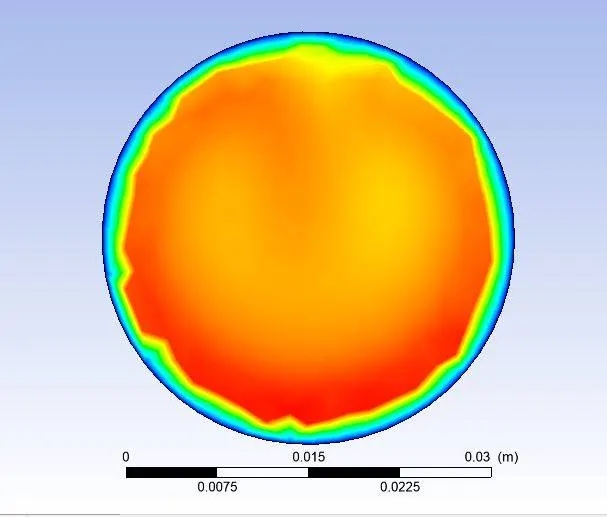
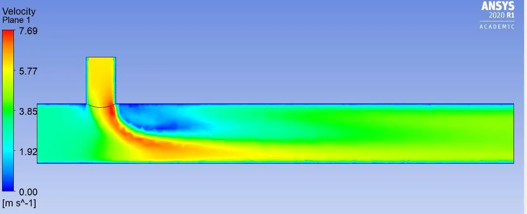
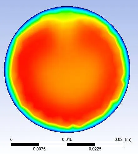
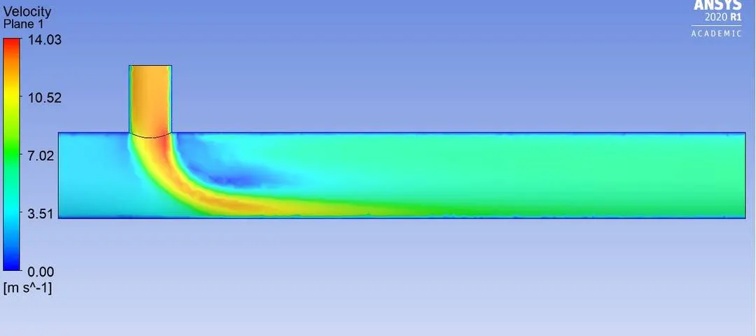
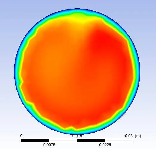
Effects of the velocity on the pipe across it's length and at the outlet
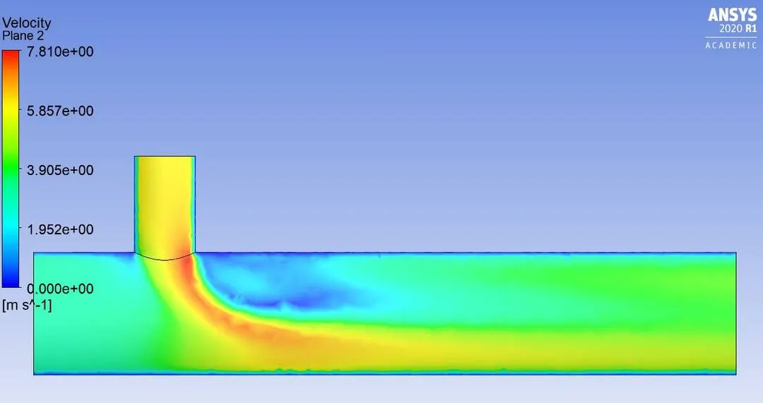
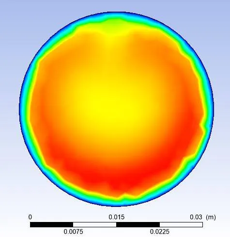
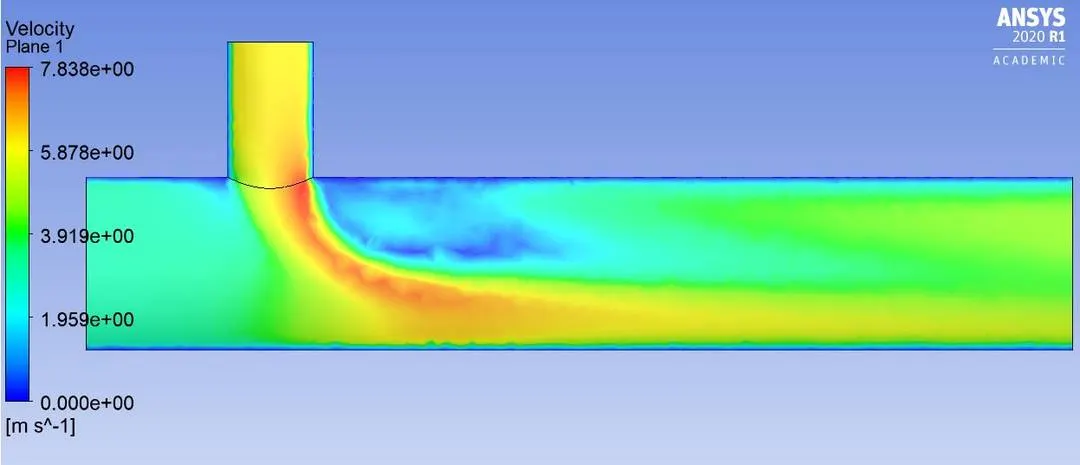
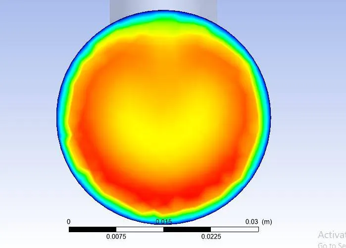
So in the above pictures, we can say that the velocity is different at every point in the mixing tee and in the outlet the at the boundary of the pipe the velocity is zero because of the shear stress.
Graphs
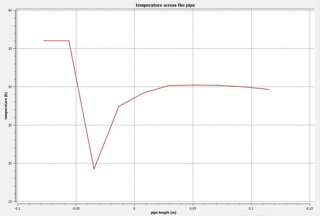
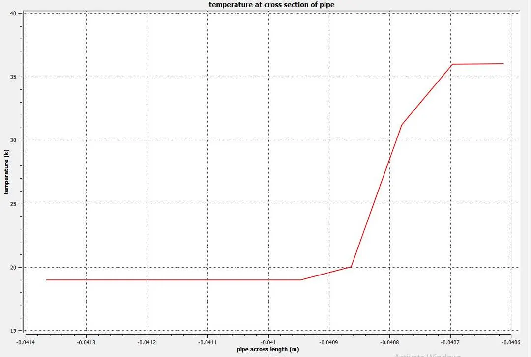
We are plotting the graph on the basis of these lines
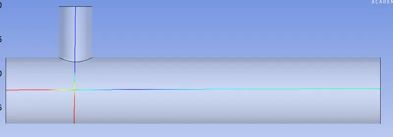
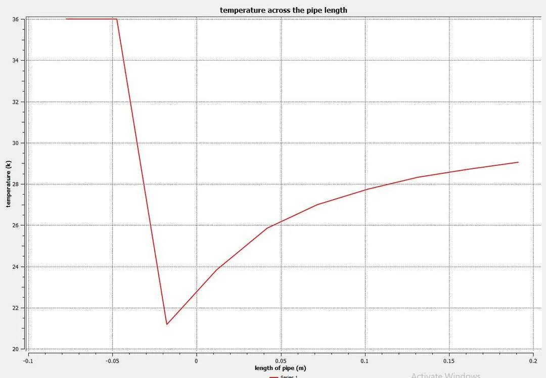
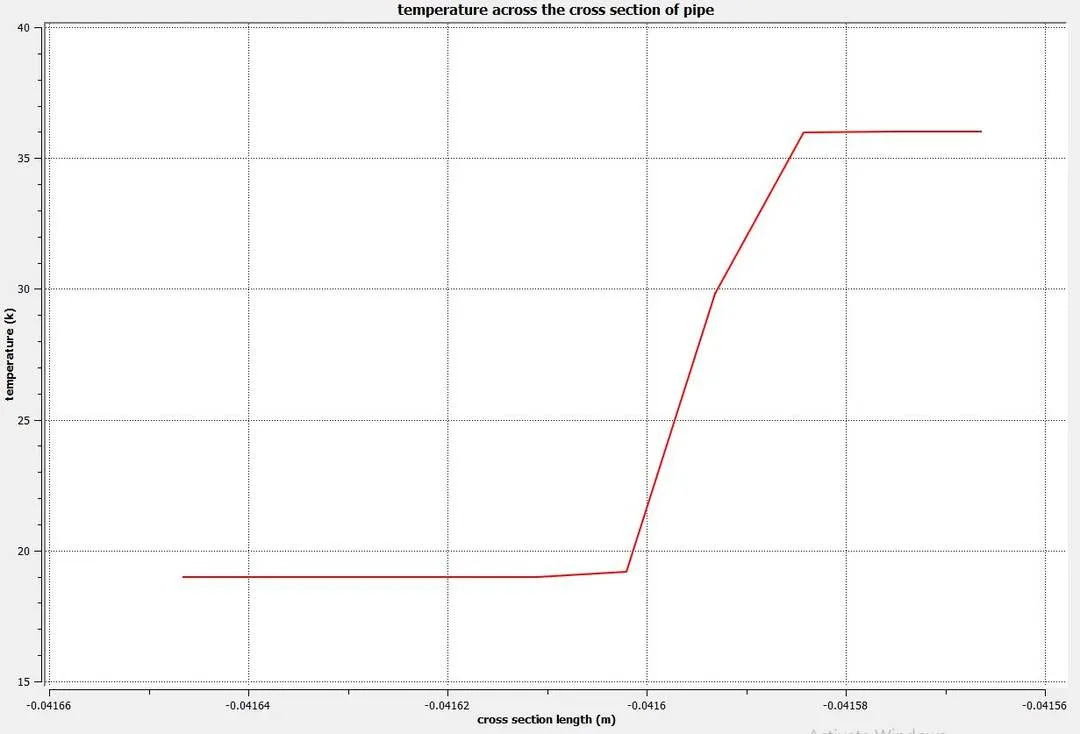
One line is across the length of the pipe and second one is across the cross-section of the pipe at the T-Junction where hot and cold air are starts mixing.
The temperature on the pipe across it's length and at the cross section(T-junction) of the pipe
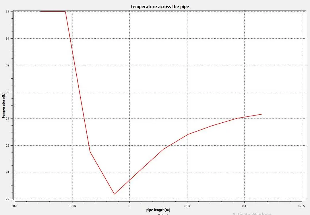
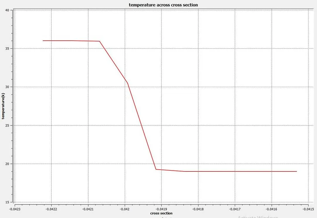
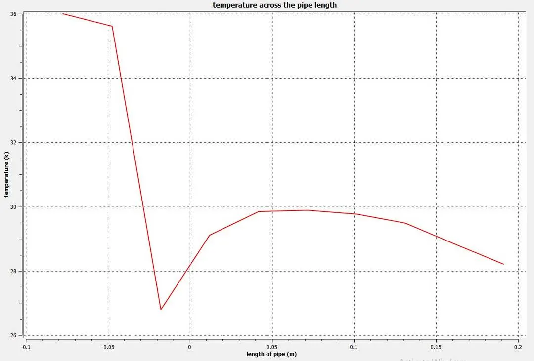
So in the graph, we can see that the temperature is high at the beginning and when it reaches the T-junction where hot and cold air starts to mix it decreases rapidly and when they start mixing temperature again increases.
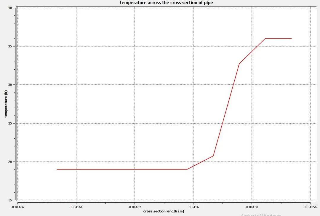
When we plot the graph of temperature and cross-section of pipe(at T-Junction) we see that at the beginning the temperature is high here the hot air is present and as the length increases the temperature decreases at the end is minimum This where cold air is entering the pipe.
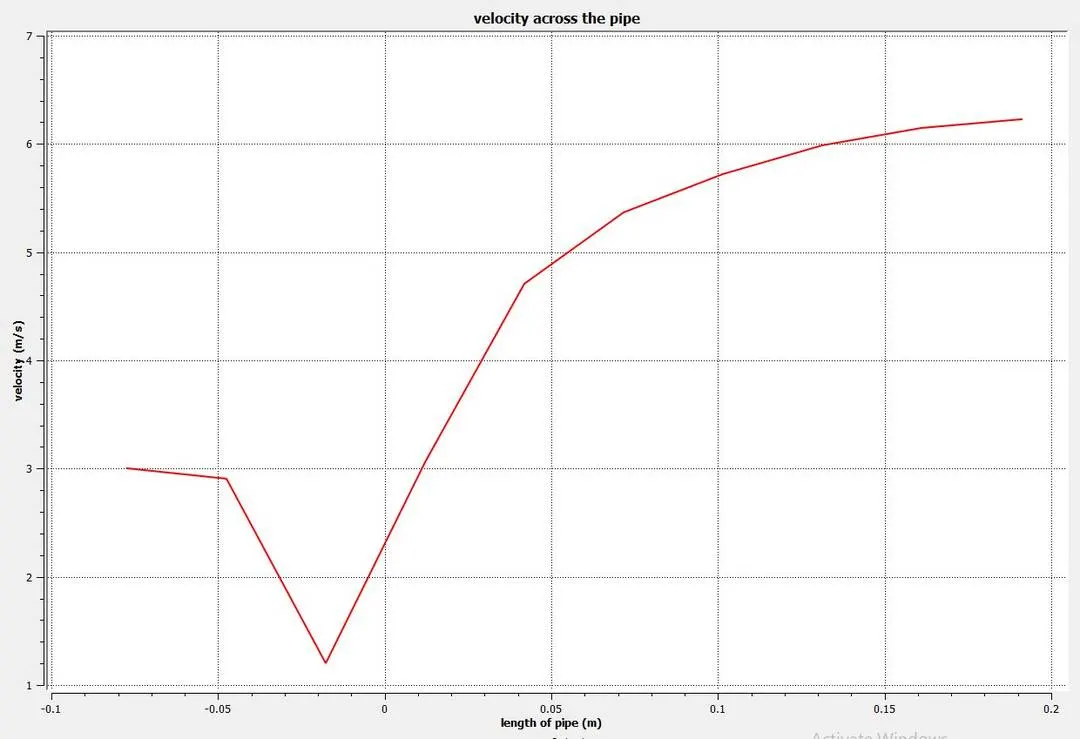
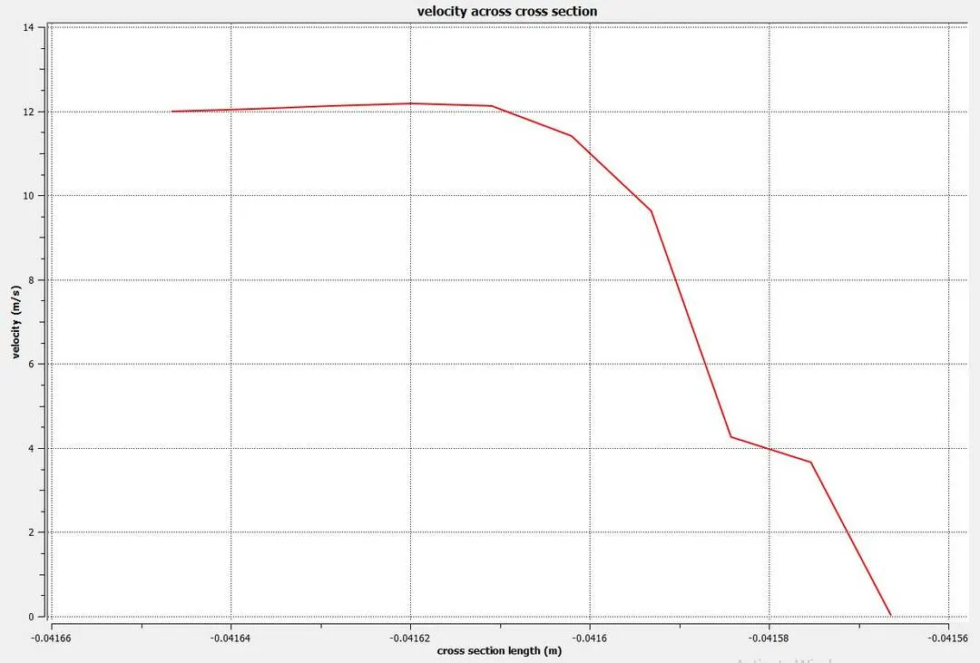
The velocity on the pipe across its length and at the cross section(T-junction) of the pipe
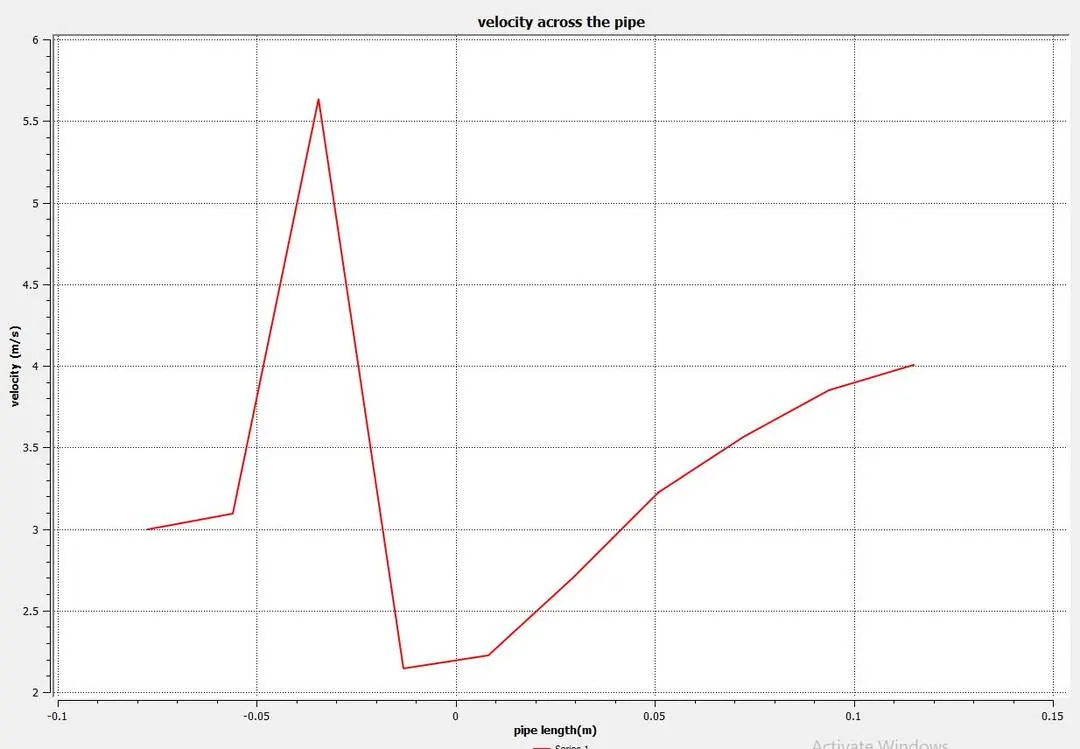
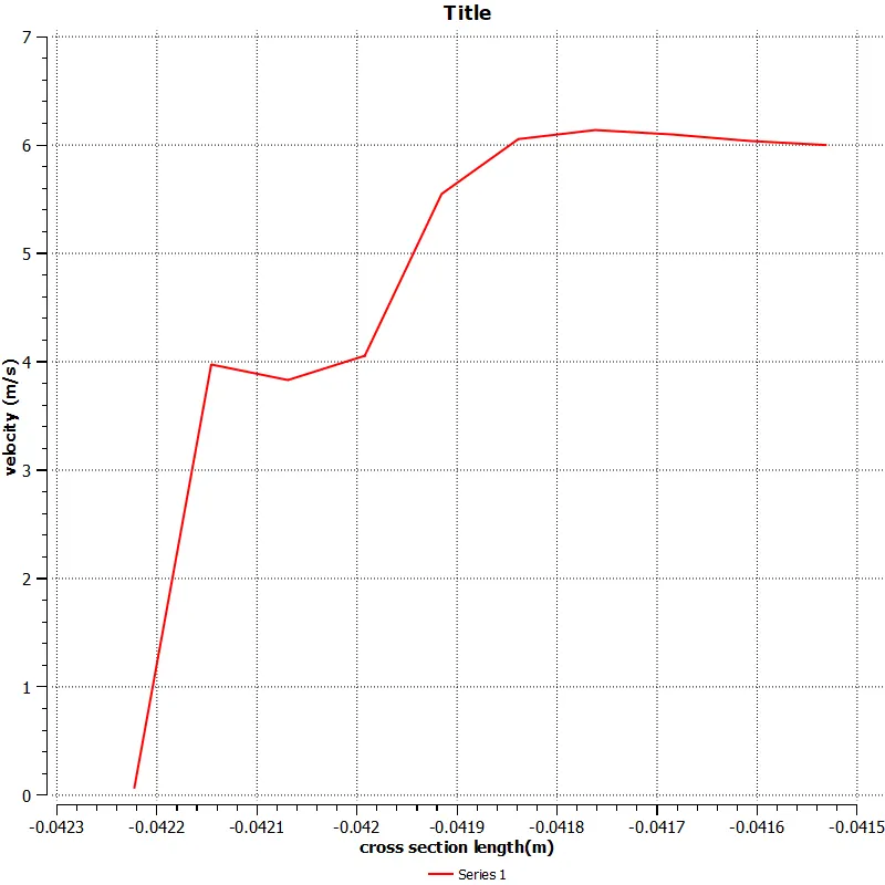
So in the graph, we can see that the velocity is 3 m/s at the beginning and when it reaches the T-junction where hot and cold air starts to mix it increases rapidly and decreases. When they start mixing velocity again increases.
When we plot the graph of velocity and cross-section of pipe(at T-Junction) we see that at the beginning the velocity is low here the hot air is present and as the length increases the velocity increases at the end is maximum this where cold air is entering the pipe.
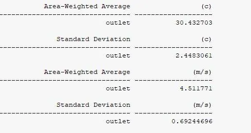
The result we get are these
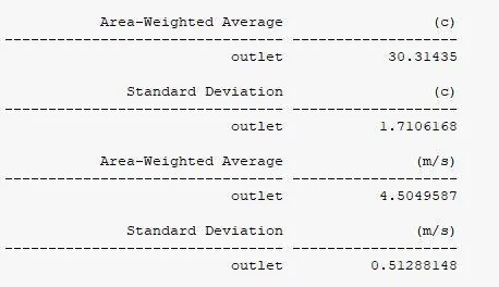
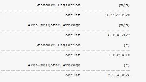
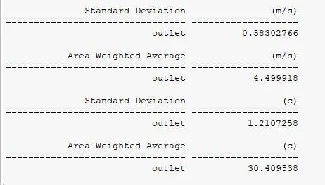
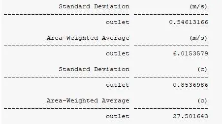
So these are the values we are getting from the reports we have created in the setUp.
Case-2
Short length pipe with momentum ratio of 2 using k-`omega` model
So in this case we have taken the element size = 0.002 m
We are going to use SST k-`omega` model
For hot air
Inlet temperature = 36 degree celcius
Inlet velocity = 3 m/s
For cold air
Inlet temperature = 19 degree celcius
Inlet velocity = 6 m/s
Solution
Residual
Temperature
Velocity
Result
Post Processing
Effects of the temperature on the pipe across it's length and at the outlet
Effects of the velocity on the pipe across it's length and at the outlet
Graphs
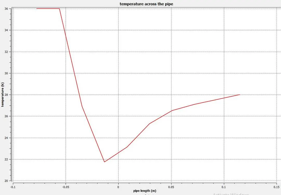
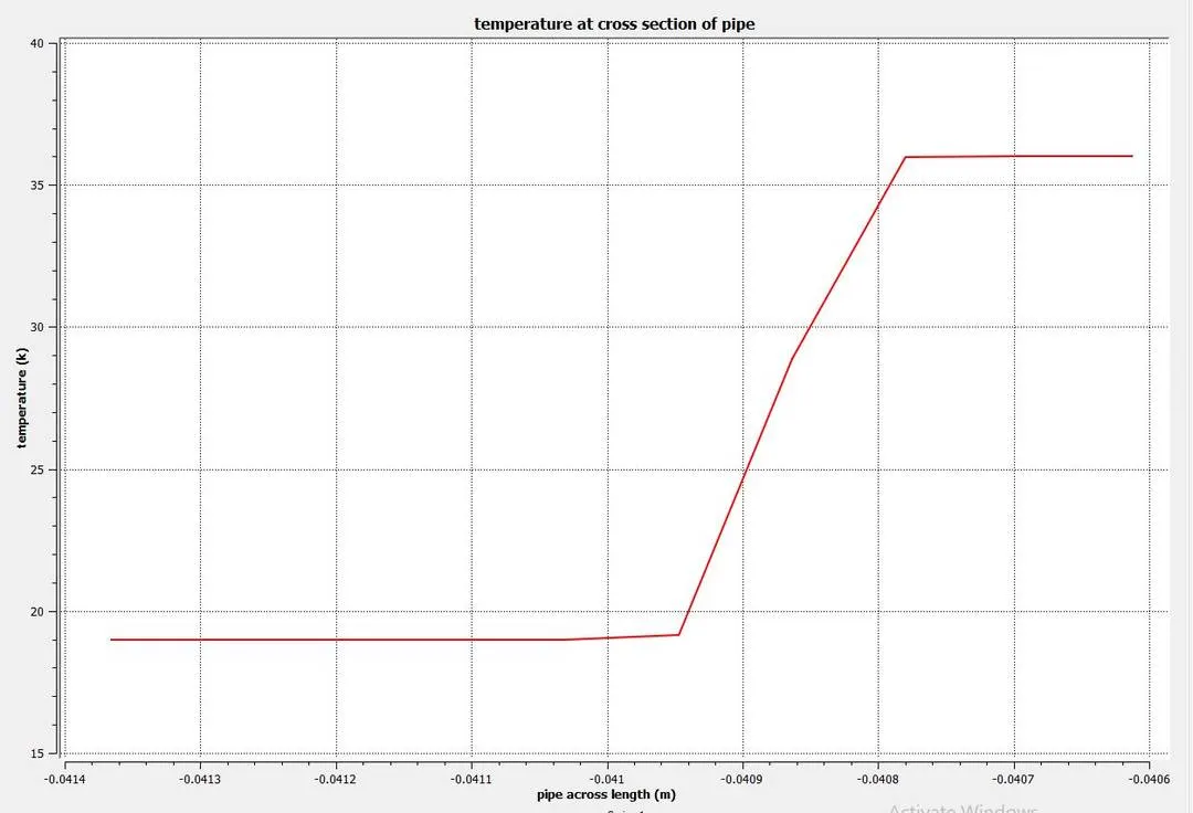
The temperature on the pipe across it's length and at the cross section(T-junction) of the pipe
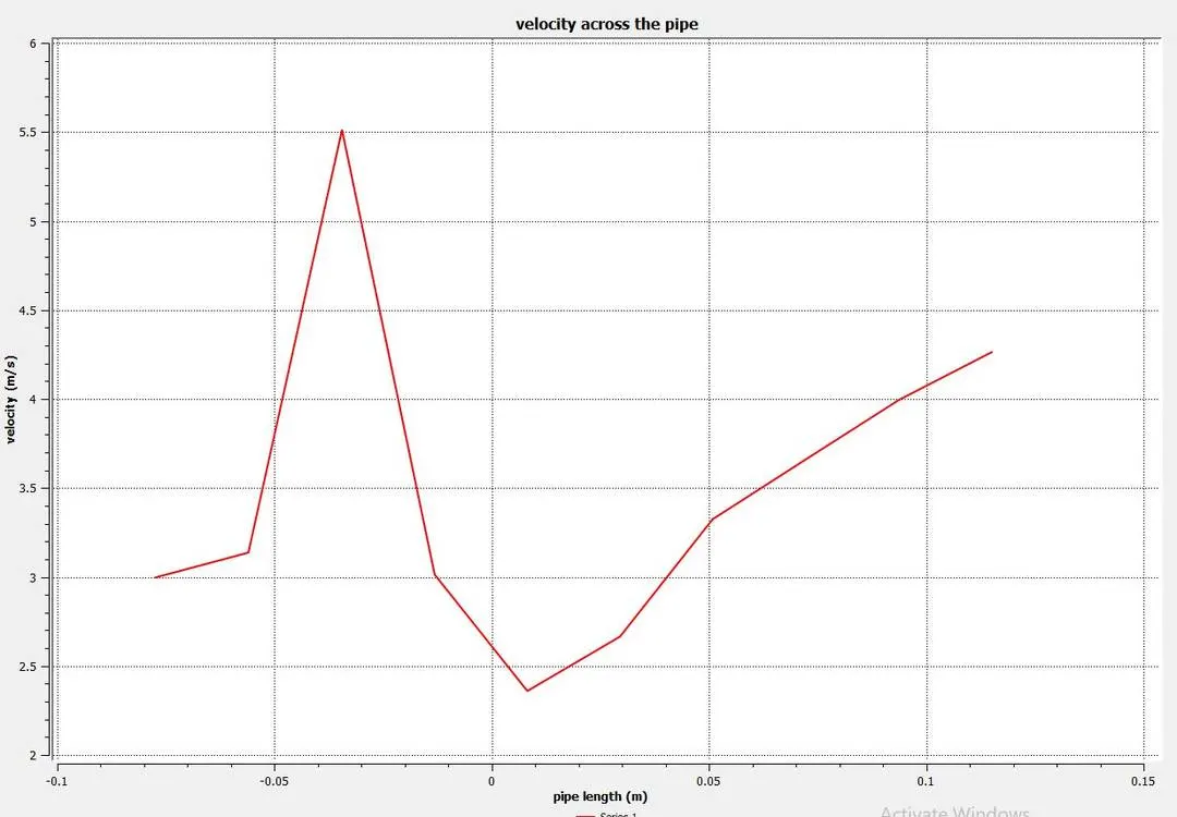
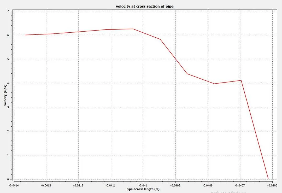
The velocity on the pipe across it's length and at the cross section(T-junction) of the pipe
The result we get are these
Case-3
Short length pipe with momentum ratio of 4 using k-`epsilon` model
So in this case we have taken the element size = 0.002 m
We are going to use realizable k-ɛ model
For hot air
Inlet temperature = 36 degree celcius
Inlet velocity = 3 m/s
For cold air
Inlet temperature = 19 degree celcius
Inlet velocity = 12 m/s
Solution
Residual
Temperature
Velocity
Result
Post Processing
Effects of the temperature on the pipe across it's length and at the outlet
Effects of the velocity on the pipe across it's length and at the outlet
Graphs
The temperature on the pipe across it's length and at the cross section(T-junction) of the pipe
The velocity on the pipe across it's length and at the cross section(T-junction) of the pipe
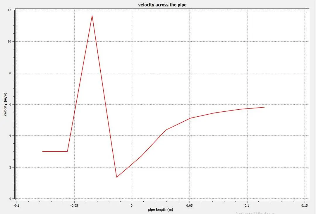
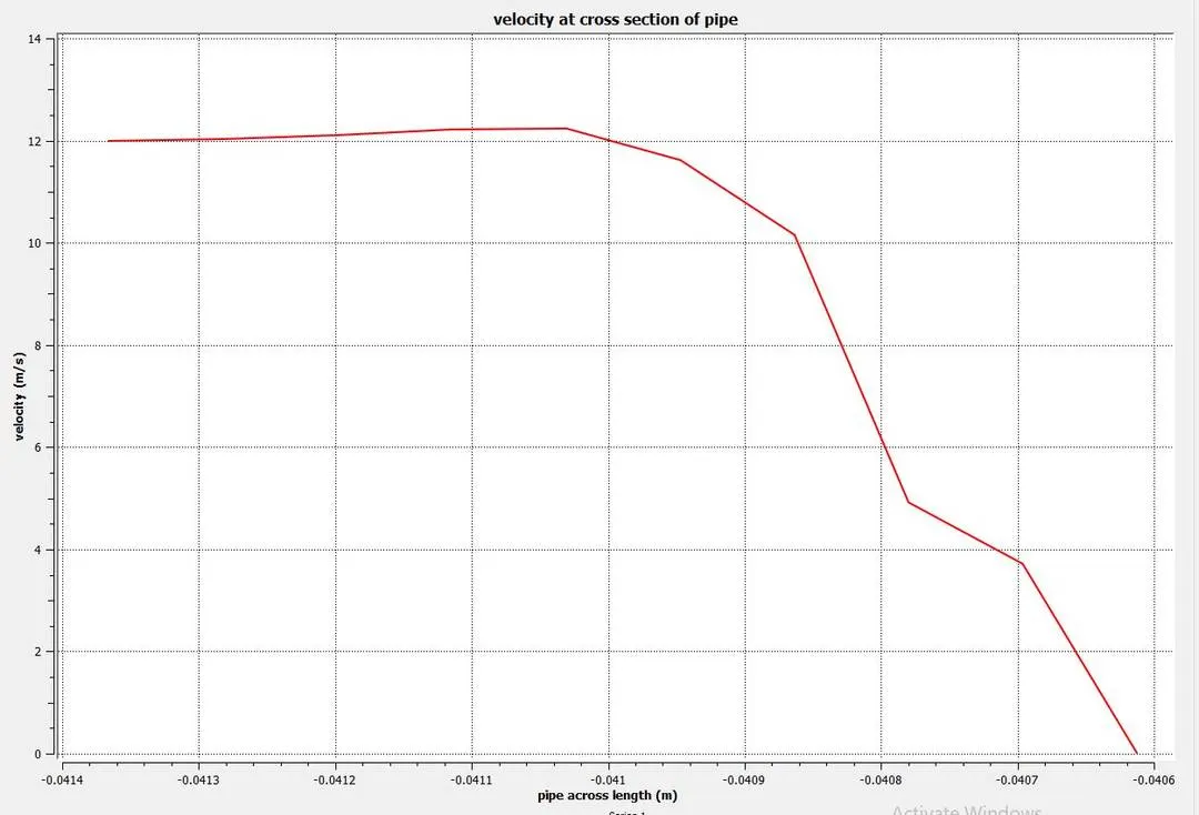
The result we get are these
Case-4
Short length pipe with momentum ratio of 4 using k-`omega` model
So in this case we have taken the element size = 0.002 m
We are going to use SST k-`omega` model
For hot air
Inlet temperature = 36 degree celcius
Inlet velocity = 3 m/s
For cold air
Inlet temperature = 19 degree celcius
Inlet velocity = 12 m/s
Solution
Residual
Temperature
Velocity
Result
Post Processing
Effects of the temperature on the pipe across it's length and at the outlet
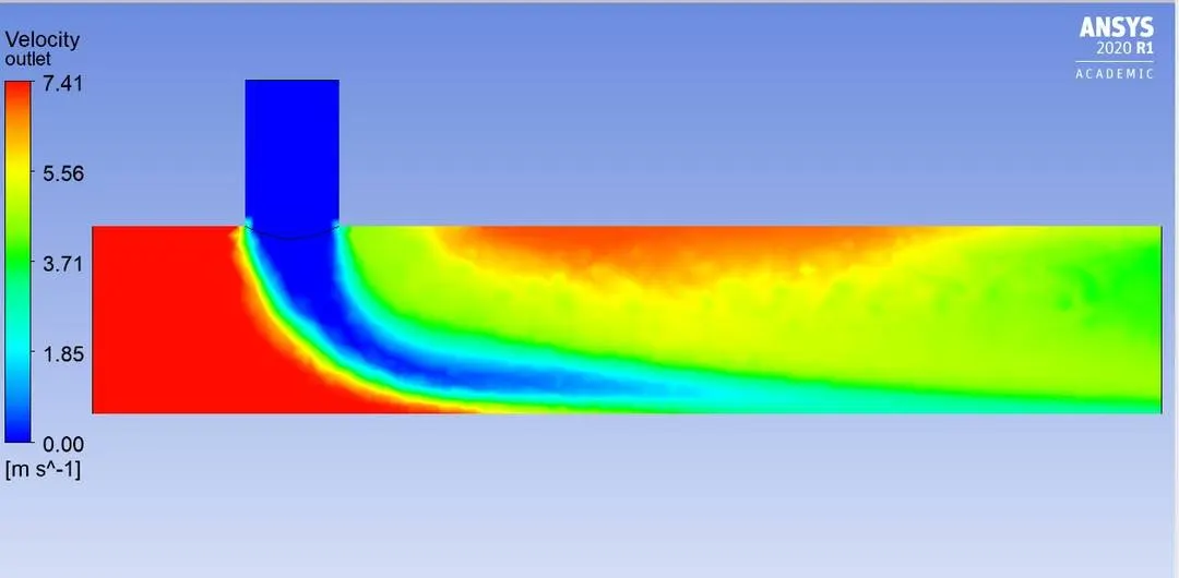
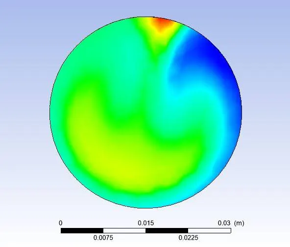
Effects of the velocity on the pipe across it's length and at the outlet
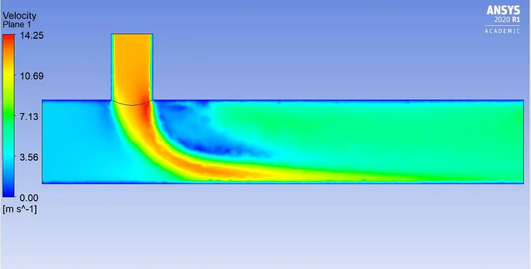
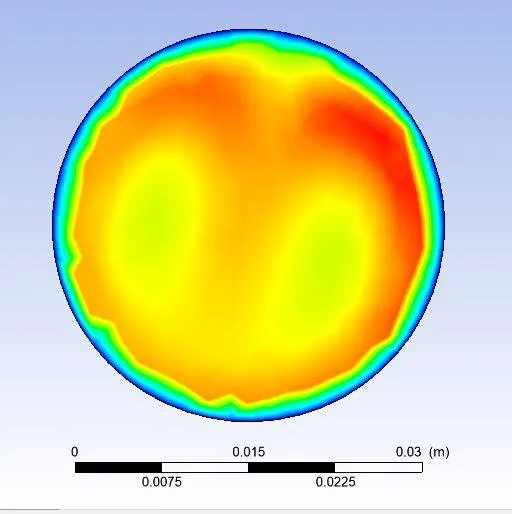
Graphs
The temperature on the pipe across it's length and at the cross section(T-junction) of the pipe
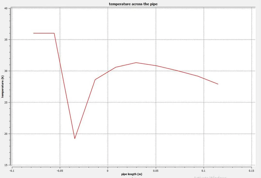
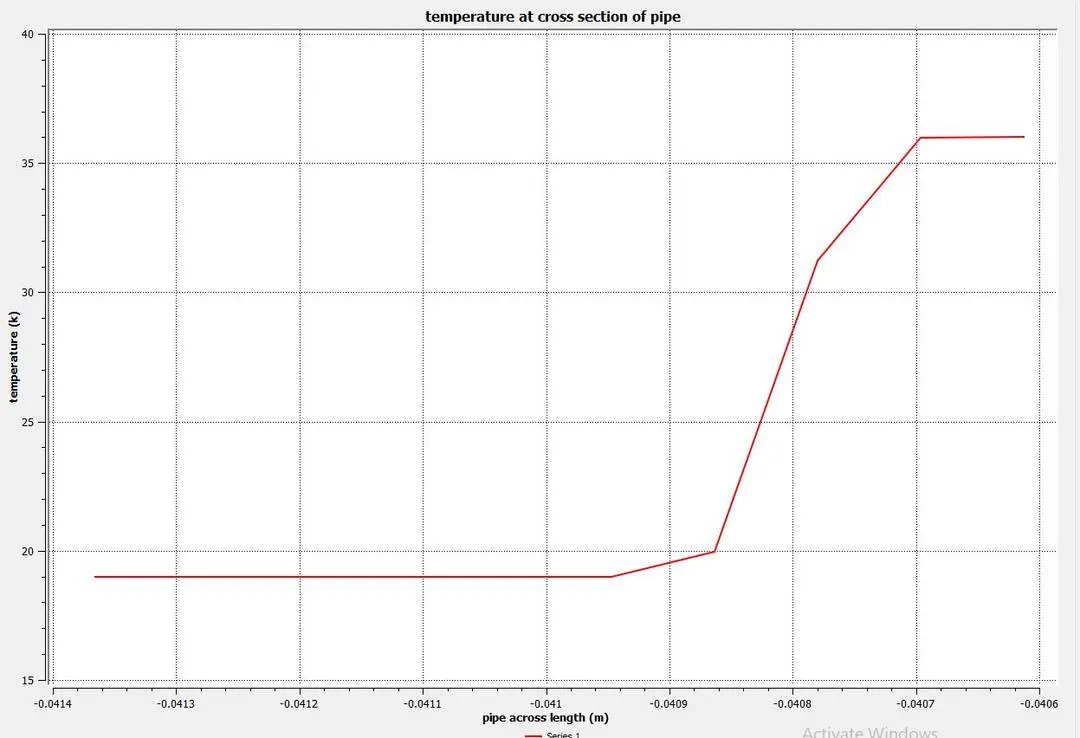
The velocity on the pipe across it's length and at the cross section(T-junction) of the pipe
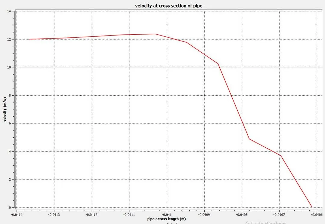
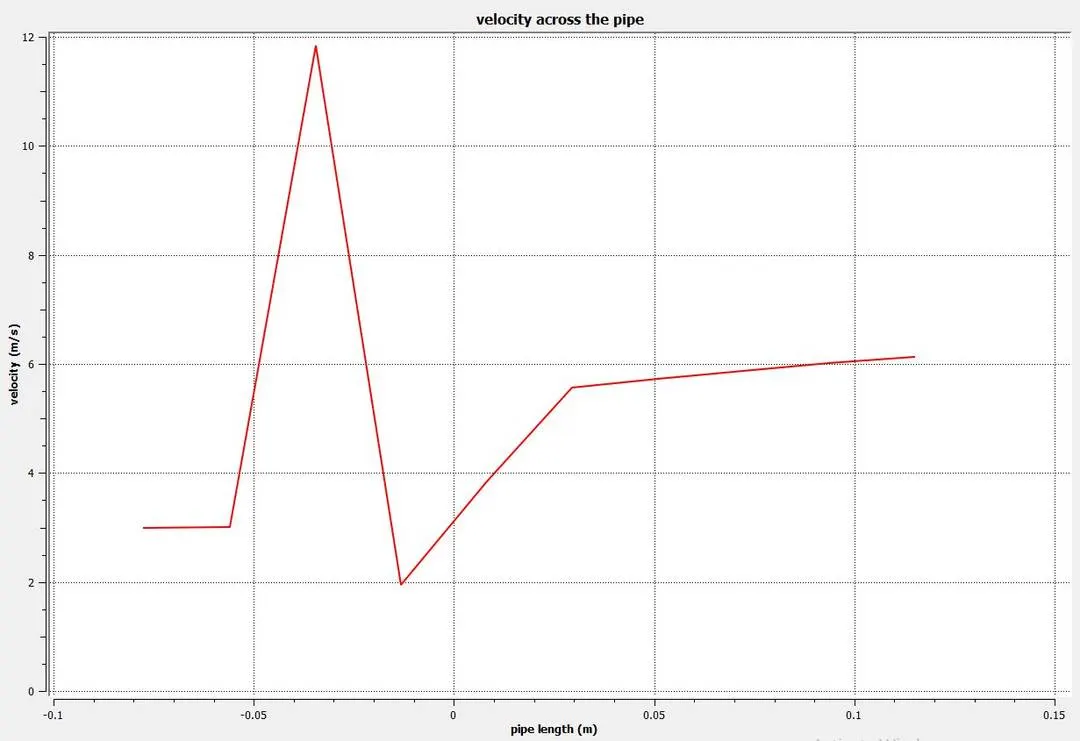
The result we get are these
Reason to choose k-`epsilon` model for the next cases
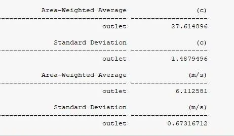
When we observe these four cases, we get the average value of the temperature at the outlet is more accurate to the analytical result when we are using k-`epsilon` model.
When we compare the results of k-`epsilon` and k-`omega` we can see that the number of iteration to get the convergence results are more in the k-`omega` model and the standard deviation is also more and less standard deviation gives us more efficient results. So k-`epsilon` model gives us more efficient results. k-`omega` model is used for low Reynolds number and Y+ value should be less than 5. But in this case our Y+ value is higher than the 15.
So from now on we are going to use k-`epsilon` model.
Case-5
Long length pipe with momentum ratio of 4 using k-`epsilon` model
So in this case we have taken the element size = 0.002 m
We are going to use realizable k-ɛ model
For hot air
Inlet temperature = 36 degree celcius
Inlet velocity = 3 m/s
For cold air
Inlet temperature = 19 degree celcius
Inlet velocity = 6 m/s
Solution
Residual
Temperature
Velocity
Result
Post Processing
Effects of the temperature on the pipe across it's length and at the outlet
Effects of the velocity on the pipe across it's length and at the outlet
Graphs
The temperature on the pipe across it's length and at the cross section(T-junction) of the pipe
The velocity on the pipe across it's length and at the cross section(T-junction) of the pipe
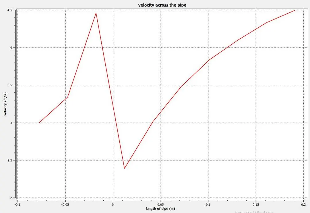
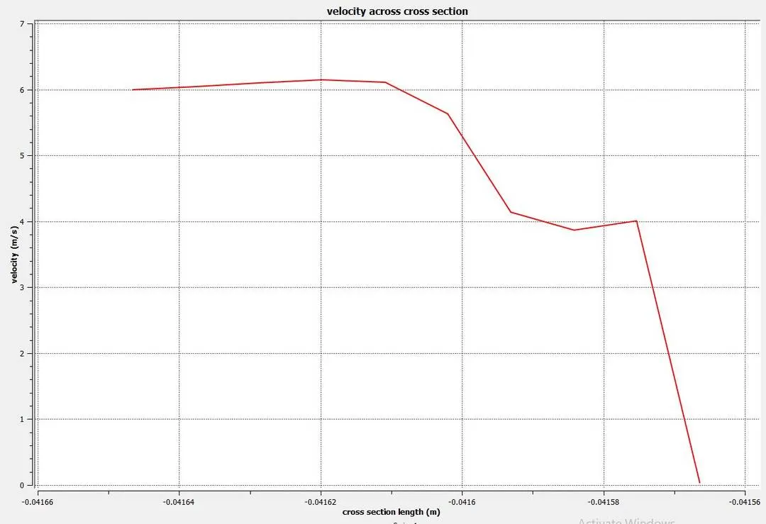
The result we get are these
Case-6
Long length pipe with momentum ratio of 4 using k-`epsilon` model
So in this case we have taken the element size = 0.002 m
We are going to use realizable k-ɛ model
For hot air
Inlet temperature = 36 degree celcius
Inlet velocity = 3 m/s
For cold air
Inlet temperature = 19 degree celcius
Inlet velocity = 12 m/s
Solution
Residual
Temperature
Velocity
Result
Post Processing
Effects of the temperature on the pipe across it's length and at the outlet
Effects of the velocity on the pipe across it's length and at the outlet
Graphs
The temperature on the pipe across it's length and at the cross section(T-junction) of the pipe
The velocity on the pipe across it's length and at the cross section(T-junction) of the pipe
The result we get are these
Comparision
| Area-Weighted Temperature (numerical) (degree Celcius) | Analytical Temperature (degree Celcius) | Standard Deviation Temperature (degree Celcius) | |
| Short length pipe with momentum ratio of 2 using k-`epsilon` model | 30.3143 | 24.6 | 1.7106 |
| Long length pipe with momentum ratio of 2 using k-`epsilon` model | 30.4095 | 24.6 | 1.2107 |
| Short length pipe with momentum ratio of 4 using k-`epsilon` model | 27.5600 | 22.4 | 1.0930 |
| Long length pipe with momentum ratio of 4 using k-`epsilon` model | 27.5016 | 22.4 | 0.8537 |
Conclusion
1. If the standard deviation is less than we can say that the result we got is more efficient.
2. When we increase the length of the pipe we got more accurate results. So we can say that with the increase of the length of the pipe we will get more accurate results.
3. When we increase the momentum ratio we got more accurate results. So we can say that with the increase in the momentum ratio we will get more accurate results.
Grid Independency
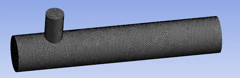
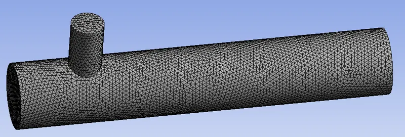
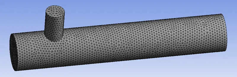
For the grid independence test, we are going to take the case-1 short length pipe with a momentum ratio of 2 with k-`epsilon` model and we are going to change the element size and we are going to compare the results.
Element size = 0.0015
Element size = 0.0020
Element size = 0.0025
Comparision
| Grid size (m) | Area-Weighted Temperature (degree Celcius) | Standard Deviation Temperature (degree Celcius) | Cell Count | Y+ | Number of iterations for convergence |
| 0.0015 | 30.3410 | 2.1079 | 211857 | 1-13 | 180-200 |
| 0.0020 | 30.3143 | 1.7106 | 106253 | 2-16 | 150-160 |
| 0.0025 | 30.2456 | 1.9183 | 60992 | 3-19 | 125-135 |
Conclusion
If we decrease the element size it should give us the more accurate result. If we take the grid element size less than 0.001 our system will not able to solve it because than number of elements will goes more than 5,00,000. So for more accurate result the grid size should be small. In this case the result does not make any sense. So it fails the grid independence test.
K-`epsilon` model gives us more accurate results if the Y+ value is higher than 30 but when in our case the y+ values don't even go to 20 so that we didn't achieve the grid independence.
When we increase the element size the number of cell decreases and it takes less number of iteration for convergence. So with the increase of the grid element size simulation will be fast but we will get less accurate results.