Genetic Algorithm
AIM:
The aim of this project is to write a program in matlab to optimise the stalagmite function and to find the global maxima of the function.
GENETIC ALGORITHM:
A genetic algorithm is a method for solving both constrained and unconstrained optimization problems based on a natural selection process that mimics biological evolution. It is a search-based optimization technique and is frequently used to find optimal or near optimal solution.
Phases in Genetic Algorithm:
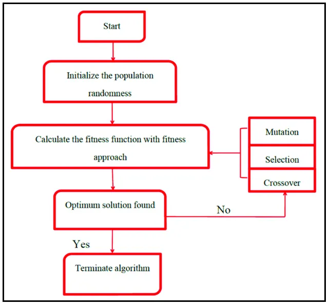
1) Initialization of population
The algorithm begins with population initialization,population is the number of sample data points taken to perform the genetic algorithm. It is very flexible as the number can be explicitly entered by the user also.
2) Fitness function
The fitness function is quantitatively measure how fit a given solution is in solving the problem. Each soluntion has a fitness score and the probability of the selection for further optimization is based on this score.
3) Selection Phase
In this step, the parent are selected from the sample data points, the main objective of the selection process is to select the highly fit individuals. More fit the individual greater is the probability of getting selected and thus evolving better individuals over time.
4) Crossover
Crossover are created by combining the vectors of a pair of parents. It is the process of taking two parents solution and producing the child form them.
5) Mutation
The algorithm creates mutation children by randomly changing the genes of individual parents. Mutation occurs to maintain diversity within population and prevent premature convergence. By default, for unconstrained problems the algorithm adds a random vector from a Gaussian distribution to the parent. For bounded or linearly constrained problems, the child remains feasible.
FLOW CHART:
SYNTAX FOR GENETIC ALGORITHM
x = ga(fun,nvars)
x = ga(fun,nvars,A,b)
x = ga(fun,nvars,A,b,Aeq,beq)
x = ga(fun,nvars,A,b,Aeq,beq,lb,ub)
x = ga(fun,nvars,A,b,Aeq,beq,lb,ub,nonlcon)
x = ga(fun,nvars,A,b,Aeq,beq,lb,ub,nonlcon,options)
x = ga(fun,nvars,A,b,[],[],lb,ub,nonlcon,IntCon)
x = ga(fun,nvars,A,b,[],[],lb,ub,nonlcon,IntCon,options)
x = ga(problem)
[x,fval] = ga(___)
[x,fval,exitflag,output] = ga(___)
[x,fval,exitflag,output,population,scores] = ga(___)

*************************************************************
x = ga(fun,nvars) finds a local unconstrained minimum, x, to the objective function, fun. nvars is the dimension (number of design variables) of fun.

x = ga(fun,nvars,A,b) finds a local minimum x to fun, subject to the linear inequalities A*x ≤ b. ga evaluates the matrix product A*x as if x is transposed (A*x').

x = ga(fun,nvars,A,b,Aeq,beq) finds a local minimum x to fun, subject to the linear equalities Aeq*x = beq and A*x ≤ b. (Set A=[] and b=[] if no linear inequalities exist.) ga evaluates the matrix product Aeq*x as if x is transposed (Aeq*x').

x = ga(fun,nvars,A,b,Aeq,beq,lb,ub) defines a set of lower and upper bounds on the design variables, x, so that a solution is found in the range lb ≤ x ≤ ub. (Set Aeq=[] and beq=[] if no linear equalities exist.)
STALAGMITE FUNCTION
The initial code for stalagmite function:
function [f]= stalagmite(input_vector)

% x and y is the input parameter
x=input_vector(1);
y=input_vector(2);

f1=(sin(5.1*pi*x+0.5)).^6;
f2=exp(-4*log(2)*((x-0.0667).^2./0.64));
f3=(sin(5.1*pi*y+0.50)).^6;
f4=exp(-4*log(2)*((y-0.0667).^2./0.64));

% Negative sign is used to reverse the plot for finding maxima
f=-(f1.*f2.*f3.*f4);
end
MAIN BODY OF GA code :
This is the initial code for generating stalagmite function through GA
clear all
close all
clc

%Defining the search space
A=linspace(0,0.6,150);
B=linspace(0,0.6,150);

% Creating 2D mesh
[xx yy]=meshgrid(A,B);

%Number of itreation
num_cases=50;

%Evaluating the stalagmite function
for i=1:length(xx)
    for j= 1:length(yy)
        input_vector(1)=xx(i,j);
        input_vector(2)=yy(i,j);
        f(i,j)=stalagmite(input_vector);
    end
end

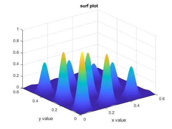
%Generating the surface plot
surf(xx,yy,-f)

% Removing the grid lines
shading interp
xlabel('x value')
ylabel('y value')
title('surf plot')
hold on

%%%%%%%%%%%%%%%%%%%%%%%%%%%%%%%%%%%%%%%%%%%%%%%%%%%%%%%%%%%%%%%%%%%%%%%%


% Study 1 : Statistical Behaviour of Unbounded input

% Calculating the study time through tic and toc command
tic

for n=1:num_cases

    % Calculating Optimised value at each iteration
    [input1, fopt1(n)]=ga(@stalagmite,2);
    xopt(n)=input1(1);
    yopt(n)=input1(2);
end
study_time_1=toc  ;      % display the time taken to evaluate

% plotting the graph
figure(1)
subplot(2,1,1)
surfc(xx,yy,-f)
hold on
shading interp
plot3(xopt,yopt,-fopt1,'marker','o','markersize',5,'markerfacecolor','r')
title('Study 1: Unbounded input')
xlabel('x')
ylabel('y')
subplot(2,1,2)
plot(-fopt1)
colorbar
xlabel('iteration')
ylabel('function max value')
hold on

%%%%%%%%%%%%%%%%%%%%%%%%%%%%%%%%%%%%%%%%%%%%%%%%%%%%%%%%%%%%%%%%%%%%%%%%

% Study 2 : Statistical Behaviour of bounded input

% Calculating the study time through tic and toc command
tic

for n=1:num_cases

    % Calculating Optimised value at each iteration
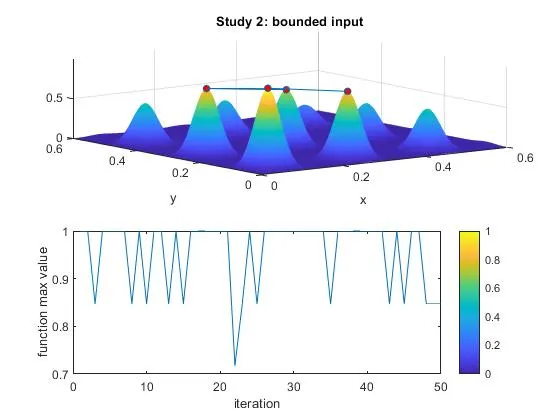
    [input2, fopt2(n)]=ga(@stalagmite,2,[],[],[],[],[0;0],[0.6;0.6]);
    xopt(n)=input2(1);
    yopt(n)=input2(2);
end
study_time_2=toc;        % display the time taken to evaluate

% plotting the graph
figure(2)
subplot(2,1,1)
surfc(xx,yy,-f);
hold on
shading interp
plot3(xopt,yopt,-fopt2,'marker','o','markersize',5,'markerfacecolor','r')
title('Study 2: bounded input')
xlabel('x');
ylabel('y');
subplot(2,1,2)
plot(-fopt2);
colorbar
xlabel('iteration')
ylabel('function max value')

%%%%%%%%%%%%%%%%%%%%%%%%%%%%%%%%%%%%%%%%%%%%%%%%%%%%%%%%%%%%%%%%%%%%%%%%

% Study 3 :  Increasing GA iteration

%options=optimoptions('ga');
options=optimoptions(@ga,'PopulationSize',500);

% Calculating the study time through tic and toc command

tic

for n=1:num_cases

    % Calculating Optimised value at each iteration
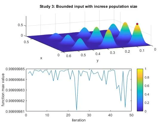
    [input3, fopt3(n)]=ga(@stalagmite,2,[],[],[],[],[0;0],[0.6;0.6],[],[],options);
    xopt(n)=input3(1);
    yopt(n)=input3(2);

end

study_time_3=toc ;      % display the time taken to evaluate

% plotting the graph
figure(3)
subplot(2,1,1)
hold on
surfc(xx,yy,-f)
hold on
shading interp
plot3(xopt,yopt,-fopt3,'marker','o','markersize',5,'markerfacecolor','r')
title('Study 3: Bounded input with increse population size')
xlabel('x');
ylabel('y');
subplot(2,1,2)
plot(-fopt3)
colorbar
xlabel('iteration')
ylabel('function max value')

fprintf('study 1: Unbounded Statistical Behaviourn')
fprintf('nThe time for study 1 is %f',study_time_1)
fprintf('nThe co-ordinates of x and y for global maxima of the function are:%f,%f',input1(1),input1(2))
fprintf('nThe global maxima of the function is :%f',-(mean(fopt1)))

fprintf('study 1: Unbounded Statistical Behaviour')
fprintf('nThe time for study 2 is %f',study_time_2)
fprintf('nThe co-ordinates of x and y for global maxima of the function are:%f,%f',input2(1),input2(2))
fprintf('nThe global maxima of the function is :%f',-(mean(fopt2)))

fprintf('study 1: Unbounded Statistical Behaviour')
fprintf('nThe time for study 3 is %f',study_time_3)
fprintf('nThe co-ordinates of x and y for global maxima of the function are:%f,%f',input3(1),input3(2))
fprintf('nThe global maxima of the function is :%f',-(mean(fopt2)))
RESULTS:
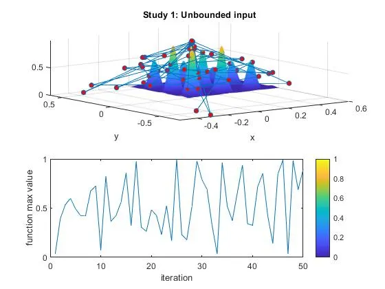
Unbounded statastical behaviour plot
From the below figure it is clear that the there is a lot of variation in optimization function value.
Bounded statistical behaviour plot:
By providing upper and lower limit in GA the search space is reduced and also variation in optimized function value is reduced.
Bounded statistical behaviour with increase population size:
By increasing the initial population size more iteration were allowed to perform thus increasing the possibility of finding better result.
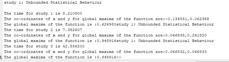
GA function output print in command window: