FINAL INDEPENDENT PROJECT
AIM:
The aim of this project is to write a MATLAB program to develop a SIR model of covid-19 to predict the future cases based on given assumption.
OBJECTIVE:
- The SIR Model is used in epidemiology to compute the amount of susceptible, infected, and
recovered people in a population. - to explain the change in the number of people needing medical attention during an epidemic.
THEORY:
Modelling diseases by using mathematical models could be considered a powerful approach since they bring us some information about the spread of a particular virus as well as estimating the peak of the pandemics by taking the necessary measures. Nowadays, most of the epidemic diseases are usually dealt with by SI, SIS, and SIR models.
Assumptions
This model is an appropriate one to use under the following assumptions :
1) The population is fixed.
2) The only way a person can leave the susceptible group is to become infected.The only way a person can leave the infected group is to recover from the disease. Once a person has recovered, the person received immunity.
3) Age, sex, social status, and race do not affect the probability of being infected.
4) There is no inherited immunity.
5) The member of the population mix homogeneously (have the same interactions with one another to the same degree).
MODELING PARAMETERS:
S- is the number of susceptibles, who are not infected but could become infected.
I- is the number of infectives. These individuals have the disease and can transmit it to the susceptibles.
R -is the number of recovered individuals. These may or may not have the disease, but they can't become infected and they can't transmit the disease to others.
The assumptions lead us to a set of differential equations.
- New infections occur as a result of contact between infectives and susceptibles. In this simple model the rate at which new infections occur is (`beta`*S*I) for some constant (`beta`).
`frac{ds}{dt}=- beta*S*I`
where,
ds/dt= Explains how to number of susceptible is changing with time
`beta`=Is the average number of transmissions from an infected person in a time period or effective contact rate of the disease
- The other process that can occur is that infective individuals can enter the removed class. We assume that this happens at the rate for some positive constant . Thus we have our other two differential equations:
`frac{dI}{dt}=beta*S*I-gamma*I`
`frac{dR}{dt}=gamma*I`
where,
`gamma`: This parameter is related to the recovery rate
`frac{dI}{dt}` explains how to number of Infected people is changing with time
`frac{dR}{dt}` explains how to number of recovered is changing with time
N=S+I+R is the total population
STEP -1:
- We are starting this approach by collecting the data from an excel sheet provided by the Government of India. http://api.covid19india.org/csv/latest/state_wise_daily.csv
-
Here, data is pre-processed by using table2array function and population (N), susceptible (S), infected (I) and recovered (R) individuals are computed. For this time, the data into excel sheet was chosen to be related to Maharashtra population.
MATLAB CODE:
%Reading the data from .csv file
time=readtable('state_wise_daily.csv','range','A2:A610');
time=table2array(time);
time=(time(1:3:end,1));
MH=readtable('state_wise_daily.csv','range','Y2:Y610');
MH=(table2array(MH));
STEP-2: Estimating 𝛽(B1) and 𝛾(K)
These parameters are computed according to above equations. 𝛽 (B1)and 𝛾(k) are computed as the mean value of their resulting vectors.
%%
%Initiallizing the variables

N=123144222;              %Total population
I=(MH(1:3:end,1))';       %No of infected people
R=(MH(2:3:end,1))';       %No of recovered people
D=(MH(3:3:end,1))';       %No of Death
S=N-I-D;                  %No of susceptible
%Taking fraction of population
s=S/N;
i=I/N;
r=R/N;


%% Finding the b and k value

B1=-1*([0 diff(s)]./(s.*i));
B1(isnan(B1))=[];
B1(isinf(B1))=[];
B1=abs(mean(B1))

K=([0 diff(r)]./i );
K(isnan(K))=[];
K(isinf(K))=[];
K=abs(mean(K))
STEP 3: Building and Plotting SIR model
A function called mco contains the differential equations, this is shown below:
function [A]=mco(t,y,B1,K)
p= B1+0.03;  % B1 value from covid.m code
q=K;   % k value from covid.m code
sus=-p*y(1)*y(2);
infec=p*y(1)*y(2)-q*y(2);
rec=q*y(2);
A=[sus infec rec]';
end
Now setting initial conditions and using ode45 and plot function, we can plot the model response.
%%
%Solving the equation
to=0:2:1000;                      %Time span
ini=[s(end) i(end) r(end)];       %Initial value
[t result]=ode45(@(t,u) mco(t,u,B1,K),to,ini);


%Plotting the prediction
figure(2)
plot(t,result(:,1),t,result(:,2),t,result(:,3),'linewidth',3);
title('SIR MODEL')
xlabel('TIME');
ylabel('Fraction of number of people')
legend('Susceptible','Infected','Recovered')
FULL CODE:
clear all;
close all;
clc;

%%
%Reading the data from .csv file
time=readtable('state_wise_daily.csv','range','A2:A610');
time=table2array(time);
time=(time(1:3:end,1));
MH=readtable('state_wise_daily.csv','range','Y2:Y610');
MH=(table2array(MH));

%%
%Initiallizing the variables

N=123144222;              %Total population
I=(MH(1:3:end,1))';       %No of infected people
R=(MH(2:3:end,1))';       %No of recovered people
D=(MH(3:3:end,1))';       %No of Death
S=N-I-D;                  %No of susceptible
%Taking fraction of population
s=S/N;
i=I/N;
r=R/N;

%%
%Plotting the current data
figure(1);

plot(time,I,'b',time,D,'r');
xlabel('No of days');
ylabel('No of people');
legend('Comfirmed cases','Deaths')
hold on

%% Finding the b and k value

B1=-1*([0 diff(s)]./(s.*i));
B1(isnan(B1))=[];
B1(isinf(B1))=[];
B1=abs(mean(B1))

K=([0 diff(r)]./i );
K(isnan(K))=[];
K(isinf(K))=[];
K=abs(mean(K))

%%
%Solving the equation
to=0:2:1000;                      %Time span
ini=[s(end) i(end) r(end)];       %Initial value
[t result]=ode45(@(t,u) mco(t,u,B1,K),to,ini);


%Plotting the prediction
figure(2)
plot(t,result(:,1),t,result(:,2),t,result(:,3),'linewidth',3);
title('SIR MODEL')
xlabel('TIME');
ylabel('Fraction of number of people')
legend('Susceptible','Infected','Recovered')
RESULTS:
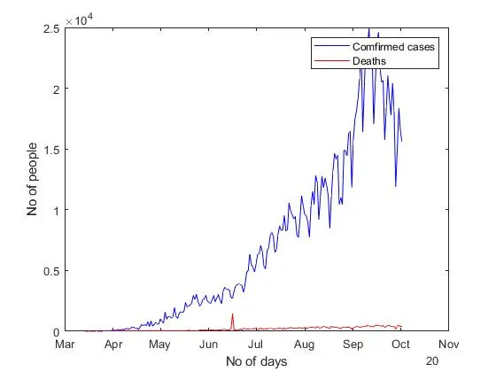
The data used till 2nd October 2020 for all these analysis.
The below result show how Covid-19 cases are rising in Maharashtra with respect to time
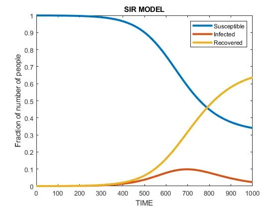
The following graph predict the future Susceptible,Infected,Recovered cases and how it changes with respect to time.
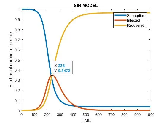
If B1(beta) is Increased i.e the average number of transmissions from an infected person in a time period or effective contact rate of the disease, more number of people comes in contact with Infected person causing a sudden rise in infectives. To avoid this Social Distancing measures can be used to prevent the spread of disease.
CONCLUSION:
Mathematical modelling theories are effective tools to deal with patterns of disease outbreaks. They provide us with useful predictions in the context of the impact of intervention in decreasing the number of infected-susceptible incidence rates.A SIR model can also assist in decision-making by making projections regarding important issues such as intervention-induced changes in the spread of disease.
References