Solving second order ODEs

AIM:

The main aim of the project is to write a MATLAB program to simulate the motion of pendulum by solving the below odinary differential equation.

THEORY:

ODE is used to describe the transient behavior of a system.The way the pendulum moves depends on the Newtons second law. When this law is written down, we get a second order Ordinary Differential Equation that describes the position of the "ball" w.r.t time. This ODE represents the equation of motion of a simple pendulum with damping

In the above equation,

g = gravity in m/s2,

L = length of the pendulum in m,

m = mass of the ball in kg,

b=damping coefficient.

FUNCTION CODE:

function [dtheta_dt]= ode_func(t,theta,b,g,l,m)

theta1=theta(1)
theta2=theta(2)
dtheta1_dt = theta2;
dtheta2_dt = -(b/m)*theta2 - (g/l)*sin(theta1);
dtheta_dt = [dtheta1_dt; dtheta2_dt]
end

MATLAB CODE:

clear all
close all
clc


b=0.05;  %damping coefficient
g=9.81;  %Gravity in m/s^2
l=1;     %length in meters 
m=1;     %mass of pendulum in kg

%initial condition
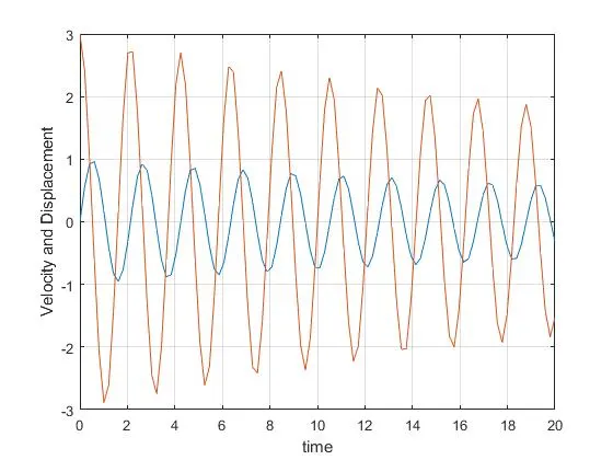
theta_0 = [0;3];         %angular velocity=3,angular displacement=0

%time points
t_span = linspace(0,20,100);

%solve ODE
[t,results] = ode45(@(t,theta) ode_func(t,theta,b,g,l,m),t_span,theta_0);

%Plotting
plot(t,results(:,1))
hold on
plot(t,results(:,2))
xlabel('time')
ylabel('Velocity and Displacement')
grid on


%animation
ct =1
for i=1:length(results(:,1))
    
    %co_ordinate of fix point of pendulum
    x0=0;
    y0=0;
    
    %co_ordinate of moving point of pendulum
    X1=l*sin(results(i,1));
    Y1=-l*cos(results(i,1));
    
    figure(2)
    plot([x0 X1],[y0 Y1],'-o','MarkerSize',10,'linewidth',3)
    axis([-2 2 -2 2])
    hold on
    plot([-1 1],[0 0],'linewidth',3,'color','r')
    hold off
    pause(0.03)
    M(ct) = getframe(gcf);
    ct=ct+1;
    
end
%creating a movie of stored frames
movie(M)
%saving the video file in '.avi' format
videofile= VideoWriter('ode_mains.avi','uncompressed AVI')
open(videofile)
writeVideo(videofile,M)
close(videofile)

RESULTS:

LINK:

https://youtu.be/cNGGig_jBF8