Project 2 - Rankine cycle Simulator
AIM:
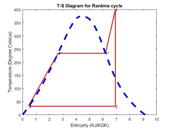
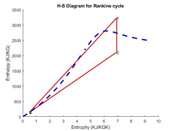
The aim of this project is to write a MATLAB program to calculate the state point of thermodynamic process and plot the T-S and H-S curve.
THEORY:
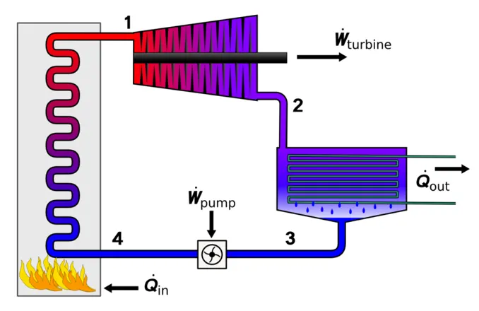
The Rankine cycle is a model used to predict the performance of steam turbine systems. The Rankine cycle is an idealized thermodynamic cycle of a heat engine that converts heat into mechanical work while undergoing phase change. The Rankine cycle operates in the following step:
1-2 Isentropic Expansion. The vapor is expanded in the turbine, thus producing work which may be converted to electricity. In practice, the expansion is limited by the temperature of the cooling medium and by the erosion of the turbine blades.
2-3 Isobaric Heat Rejection. The vapor-liquid mixture leaving the turbine is condensed at low pressure. The pressure of the vapor is well below atmospheric pressure, approaching the saturation pressure of the operating fluid at the cooling water temperature.
3-4 Isentropic Compression. The pressure of the condensate is raised in the feed pump. Because of the low specific volume of liquids, the pump work is relatively small and often neglected in thermodynamic calculations.
clear all
close all
clc

disp('RANKINE CYCLE SIMULATOR');
disp('1-2 = Isentropic expansion in the turbine');
disp('2-3 = Constant Pressure heat rejection by the condensor');
disp('3-4 = Isentropic compression in the pump');
disp('4-1 = Constant pressure heat addition by the boiler');


%Input Parameter
P1= input('Enter the inlet pressure at the turbine (in bars): ');
T1=input('Enter the inlet temperature at the turbine (in degree celsius):');
P2=input('Enter the pressure at the condenser (in bars): ');
disp(' RESULTS')


%Calculation at state point 1

%s_pT	Specific entropy as a function of pressure and temperature
s1=XSteam('s_pT',P1,T1);            %Entrophy(1)

%h_pT	Entalpy as a function of pressure and temperature.'
h1=XSteam('h_pT',P1,T1);            %Enthalphy(1)


%Calculation at state point 2
s2=s1;                               %Entrophy(2)
%sL_p	Saturated liquid entropy
%sV_p	Saturated vapour entropy
sf2=XSteam('sL_p',P2);
sg2=XSteam('sV_p',P2);
sfg2=sg2-sf2;
x2=(s1-sf2)/sfg2;                  %Dryness factor
T2=XSteam('T_ps',P2,s2);           %Temperature(2)
hf2=XSteam('hL_p',P2);
hg2=XSteam('hV_p',P2);
h2=hf2+(x2*(hg2-hf2));             %Enthalphy(2)

%Calculation at state point 3
P3=P2;
s3=XSteam('sL_p',P3);              %Entrophy(3)
h3=XSteam('hL_p',P3);              %Enthalphy(3)
T3=XSteam('Tsat_p',P3);            %Temperature(3)

%calculation at state point 4
v4=XSteam('vL_p',P3);
P4=P1;
wp=v4*(P4-P3)*100;
s4=s3;                             %Entrophy(4)
h4=wp+h3;                          %Enthalphy(4)
cp4=XSteam('cpL_p',P3);
cv4=XSteam('cvL_p',P3);
gamma=(cp4/cv4);
g=(gamma-1)/gamma;
T4=T3*((P4/P3)^g);                 %TEmperature(4)


%Turbine work
wt=h1-h2;

%Pump work
wp1=h4-h3;

%Net work
w_net=wt-wp;

%Heat in and out of the system
q_in=h1-h4;
q_out=h2-h3;

%Calculation of thermal efficiency
n=w_net/q_in;
np=n*100;

%Calculation of back work ratio
Bw_ratio=wp1/wt;

%Calculation of Specific heat consumption
ssc=3600/w_net;

%plotting all the thermodynamic process
figure(1)
plot([s1 s2],[T1 T2],'linewidth',2,'color','r')      %process1-2
hold on
plot([s2 s3],[T2 T3],'linewidth',2,'color','r')      %process2-3
plot([s3 s4],[T3 T4],'linewidth',2,'color','r')      %process 3-4

tf=XSteam('TSat_p',P4);
sf=XSteam('sL_T',tf);
plot([s4,sf],[T4,tf],'linewidth',2,'color','r')      %process 4-4'


sq=XSteam('sL_T',tf);
plot([sf,sq],[tf,tf],'linewidth',2,'color','r')        %process 4'-1'

sg_sat=XSteam('sV_p',P1)
plot([sq sg_sat],[tf,tf ],'linewidth',2,'color','r')   %process 1'-1
plot([sg_sat s1],[tf,T1 ],'linewidth',2,'color','r')

%Plotting the liquid and vapor curve
temp1=linspace(0,400,1000);
for i=1:length(temp1)
    aa(i)=XSteam('sL_T',temp1(i));
    bb(i)=XSteam('sV_T',temp1(i));
end

plot(aa,temp1,'linewidth',4,'linestyle','- -','color','b')
hold on
plot(bb,temp1,'linestyle','- -','linewidth',4,'color','b')
xlabel('Entrophy (KJ/KGK)')
ylabel('Temperature (Degree Celsius)')
title('T-S Diagram for Rankine cycle')
text(s1,T1,'1')
text(s2,T2,'2')
text(s3,T3,'3')
text(s4,T4,'4')
text(sf,tf,'4*')
text(sg_sat,tf,'1*')

%plotting all the thermodynamic process for h-s diagram
figure(2)
hold on
plot([s1 s2],[h1 h2],'linewidth',2,'color','r')     %process 1-2

plot([s2 s3],[h2 h3],'linewidth',2,'color','r')     %process 2-3

plot([s3 s4],[h3 h4],'linewidth',2,'color','r')     %process 3-4
plot([s4 s1],[h4 h1],'linewidth',2,'color','r')


%Plotting the liquid and vapour curve
temp1=linspace(0,400,1000);
for i=1:length(temp1)
    aa1(i)=XSteam('hL_T',temp1(i));
    bb2(i)=XSteam('hV_T',temp1(i));
end
hold on
plot(aa,aa1,'linewidth',3,'linestyle','- -','color','b')

plot(bb,bb2,'linestyle','- -','linewidth',3,'color','b')
xlabel('Entrophy (KJ/KGK)')
ylabel('Enthalpy (KJ/KG)')
title('H-S Diagram for Rankine cycle')
text(s1,h1,'1')
text(s2,h2,'2')
text(s3,h3,'3')
text(s4,h4,'4')
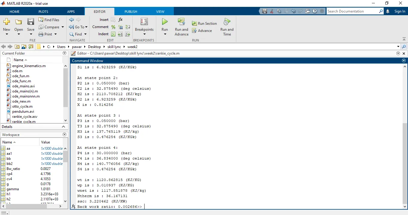
%Printting the output

fprintf('At state point 1:\n')
fprintf('P1 is : %f (bar)',P1)
fprintf('\nT 1is : %f (deg celsius)',T1)
fprintf('\nH1 is : %f (KJ/kg)',h1)
fprintf('\nS1 is : %f (KJ/KGk)',s1)

fprintf('\n\nAt state point 2: \n')
fprintf('P2 is : %f (bar)',P2)
fprintf('\nT2 is : %f (deg celsius)',T2)
fprintf('\nH2 is : %f (KJ/kg)',h2)
fprintf('\nS2 is : %f (KJ/KGk)',s2)
fprintf('\nX is : %f ',x2)

fprintf('\n\nAt state point 3 : \n')
fprintf('P3 is : %f (bar)',P3)
fprintf('\nT3 is : %f (deg celsius)',T3)
fprintf('\nH3 is : %f (KJ/kg)',h3)
fprintf('\nS3 is : %f (KJ/KGk)',s3)

fprintf('\n\nAt state point 4: \n')
fprintf('P4 is : %f (bar)',P4)
fprintf('\nT4 is : %f (deg celsius)',T4)
fprintf('\nH4 is : %f (KJ/kg)',h4)
fprintf('\nS4 is : %f (KJ/KGk)',s4)


fprintf('\n\nwt is : %f (KJ/KG)',wt)
fprintf('\nwp is : %f (KJ/KG)',wp)
fprintf('\nwnet is : %f (KJ/kg)',w_net)
fprintf('\nNtherm is : %f ',np)
fprintf('\nssc: %f (KJ/KW)',ssc)
fprintf('\nBack work ratio: %f',Bw_ratio)
CONCLUSION:
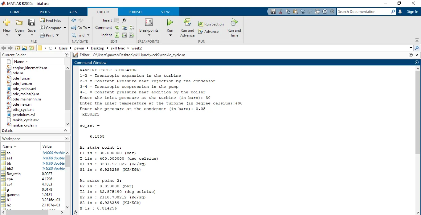
All the state points of the Rankine cycle is calculated for performance parameters along with plots for T-S and H-S diagram.