Project 1 - Parsing NASA thermodynamic data

AIM:
The main of this project is to write a matlab program for parsing the data in NASA_THERMO data file and to extract the temperature co-efficient for different species and plot thermodynamic properties like specific heat, entropy and enthalpy. Also find the molecular weigth of each species.

THEORY :

Parsing a file means reading in a data stream of some sort and building an in memory model of the semantic content of that data. This aims at facilitating perfoming some kind of transformation on the data. Here data is extracted from the file and transform into suitable plot for easy readable.

FORMULA:

At various temperature the values of Enthalpy, Entropy and specific heat is calculated to analyze the thermodynamic process. In the above data NASA came up with polynomials that can be used to evaluate thermodynamic properties such as Cp,H,S. They have documented the coefficient that are required to evaluate these polynomials for different species.

For calculating enthalphy .entropy and specific heat following formula are used:

where,

cp=specific heat

H= Enthaphy

S=Entropy

a1-a7= low temperature co-efficient

a8-a14= high temperature co-efficient

T= temperature

STEPS:

1. In the first step all the variable in worspace and plot generated are closed.
2. 'THERMO.data' file is open and saved in the 'f1' variable
3. to read the 1st line 'fgetl' command is used.
4. BY scanning the next line the data is stored in the 'temp' .
5. The data in the 'temp' variable is distributed.
6. 'for' loop is used to read all the 53 species data
7. 'strsplit' is used to split the string at whitespace to extract the species names.
8. In order to read the co-efficient string 'E ' is find with 'strfind' command and number are incremented to get the exact value of co-efficient. It is then converted into numbers.
9. 'mkdir' command is used to create a folder where plots and figures are saved.
10. Specific heat ,Entrophy,Enthalphy is calculated for low and high temperature co-efficient.
11. Plots are generated and saved in above created folder by using 'cd' commands.

MATLAB CODE:

clear all
close all
clc


f1=fopen('THERMO.dat','r');          %Reading the thermo file
file_header=fgetl(f1);               %Reading the header line 

temp=fscanf(f1,'%f',[1,3]);          %scaning the next line of 1st row and 3rd column

% assignning the variable for the above scanned value
global_low_temp=temp(1);
global_mid_temp=temp(2);
global_high_temp=temp(3);

%Reading the next 4 line

fgetl(f1);
fgetl(f1);
fgetl(f1);
fgetl(f1);

for i=1:53
    
    species_row=fgetl(f1) ;               % assigning variable to row having species name
    u=strsplit(species_row,' ');          % split string at whitespace into u
    species=(u{1});
   
    % Finding local temperature
    u1=strfind(species_row,'G');  
    temp_values=species_row(u1+4:length(species_row));
    B=strsplit(temp_values,' ');
    
    local_low_temp=str2double(B{1});
    local_high_temp=str2double(B{2});
    local_mid_temp=str2double(B{3});
    
    %calculation of temperature coefficient of 1st line(a1-a5)
    co1=fgetl(f1);
    
    z1=strfind(co1,'E')  ;                 % finding string'E' in co1 line
    
    % Temperature co-efficient
    a1=str2double(co1(1:z1(1)+3));
    a2=str2double(co1(z1(1)+4:z1(2)+3));
    a3=str2double(co1(z1(1)+4:z1(2)+3));
    a4=str2double(co1(z1(1)+4:z1(2)+3));
    a5=str2double(co1(z1(1)+4:z1(2)+3));
      
    
    %calculation of temperature coefficient of 2nd line(a6-a10)
    co2=fgetl(f1);
    
    z2=strfind(co2,'E');                   % finding string'E' in co2 line
    
    %Temperature co-efficient
    a6=str2double(co2(1:z2(1)+3));
    a7=str2double(co2(z2(1)+4:z2(2)+3));
    a8=str2double(co2(z2(2)+4:z2(3)+3));
    a9=str2double(co2(z2(3)+4:z2(4)+3));
    a10=str2double(co2(z2(4)+4:z2(5)+3));
    
     %calculation of temperature coefficient of 3rd line(a11-a14)
    co3=fgetl(f1);
    
    z3=strfind(co3,'E');                  % finding string'E' in co3 line
    
    %Temperature co-efficient
    a11=str2double(co3(1:z3(1)+3));
    a12=str2double(co3(z3(1)+4:z3(2)+3));
    a13=str2double(co2(z3(2)+4:z3(3)+3));
    a14=str2double(co2(z3(3)+4:z3(4)+3));
    
    %Creating folder
    mkdir(['c:\users\pawar\Desktop\skill lync\week4\sp\',species]);
   
    
    % local temperature range
    T=linspace(local_low_temp,local_high_temp,100);
    R=8.314;
    
    
    for n=1:length(T)
    %a1-a7=high temperature co-efficient
    %a8-a14=low temperature co-efficient
    
    %calculating specific heat,enthalpyand entropy
     if T(n)>local_high_temp  
         
         %high temperature co-efficient
         c_p=(a1+a2.*T+a3.*T.^2+a4.*T.^3+a5.*T.^4)*R;
         H=(a1+(a2.*T)./2+(a3.*T.^2)./3+(a4.*T.^3./4)+(a5.*T.^4)./5+a6./T)*R.*T;
         S=((a1.*log(T))+(a2.*T)+((a3.*T.^2)/2)+(a4.*T.^3)./3+(a5.*T.^4)./4 +a7).*R;
     else
         
         %low temperature co-efficient
         c_p=(a8+a9.*T+a10.*T.^2+a11.*T.^3+a12.*T.^4).*R;
         H=(a8+(a9.*T)./2+(a10.*T.^2)./3+(a11.*T.^3)./4+(a12.*T.^4)./5+a13./T)*R.*T;
         S=(a8.*log(T)+a9.*T+(a10.*T.^2)./2+(a11.*T.^3)./3+(a12.*T.^4)./4 +a14)*R;
     end
     
    end

%plotting the graph

figure(1);
plot(T,c_p);
title(species)
xlabel('Temperature')
ylabel('Specific heat')

figure(2);
plot(T,H);
title(species)
xlabel('Temperature')
ylabel('Enthalpy')

figure(3);
plot(T,S);
title(species)
xlabel('Temperature')
ylabel('Entropy')

%changing the directory and saving the file
s=(['c:\users\pawar\Desktop\skill lync\week4\sp\',species]);
cd(s);
saveas(1,'specific heat1.jpg');
saveas(2,'enthapy1.jpg');
saveas(3,'entropy1.jpg');


%molecular_weigth_calculation

elements=['H','C','O','N','A'];
atomic_weigth=[1.0079 12.01107 15.999 14.0067 39.948];
mol_weigth=0;
for y=1:length(species)
    for p=1:length(elements)
        if strcmp(species(y),elements(p))
            mol_weigth=mol_weigth+atomic_weigth(p);
            c=p;
        end
    end
g=str2double(species(y));
if g>1
    mol_weigth=mol_weigth+atomic_weigth(c)*(g-1);
    
end

end

fprintf('molecular weigth of %s:%f \n ',species,mol_weigth );




end

RESULTS:

Plots of O2

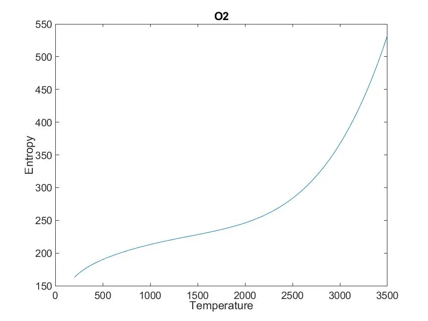
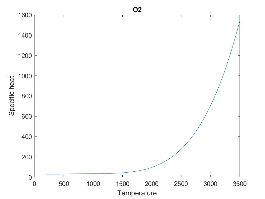
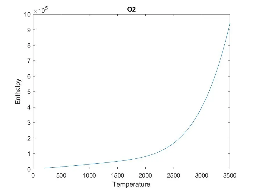
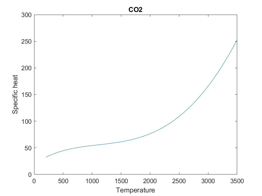
Plots of CO2

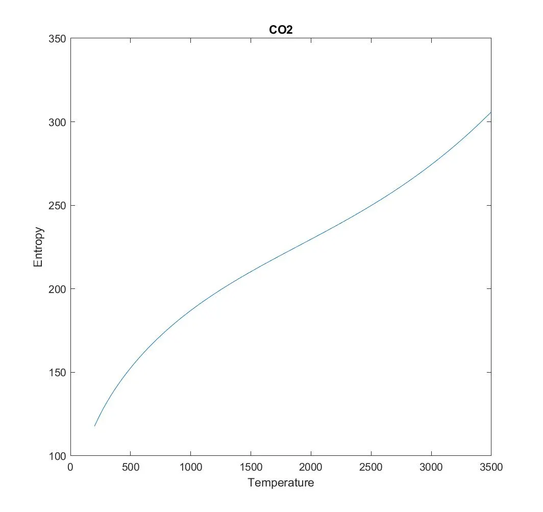
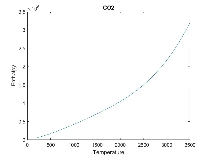
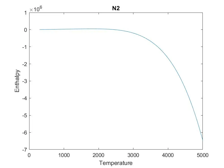
Plots of N2

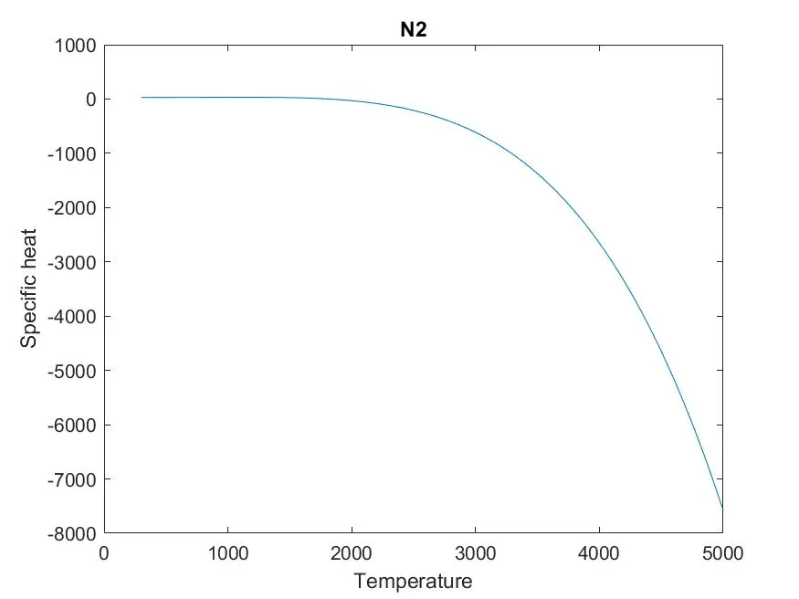
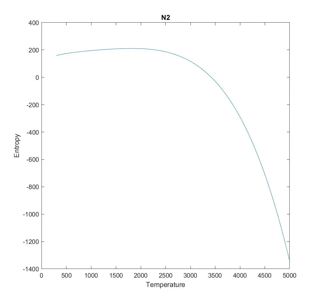
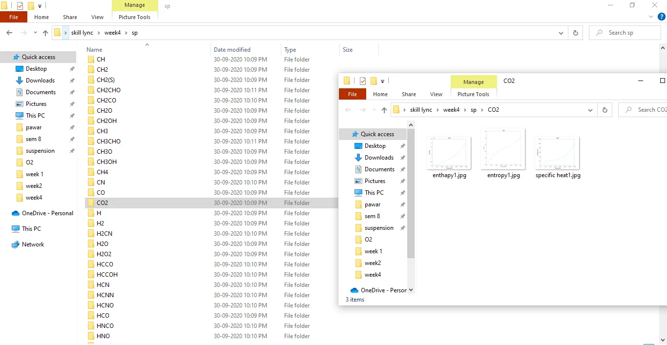
Screenshot of species folder :

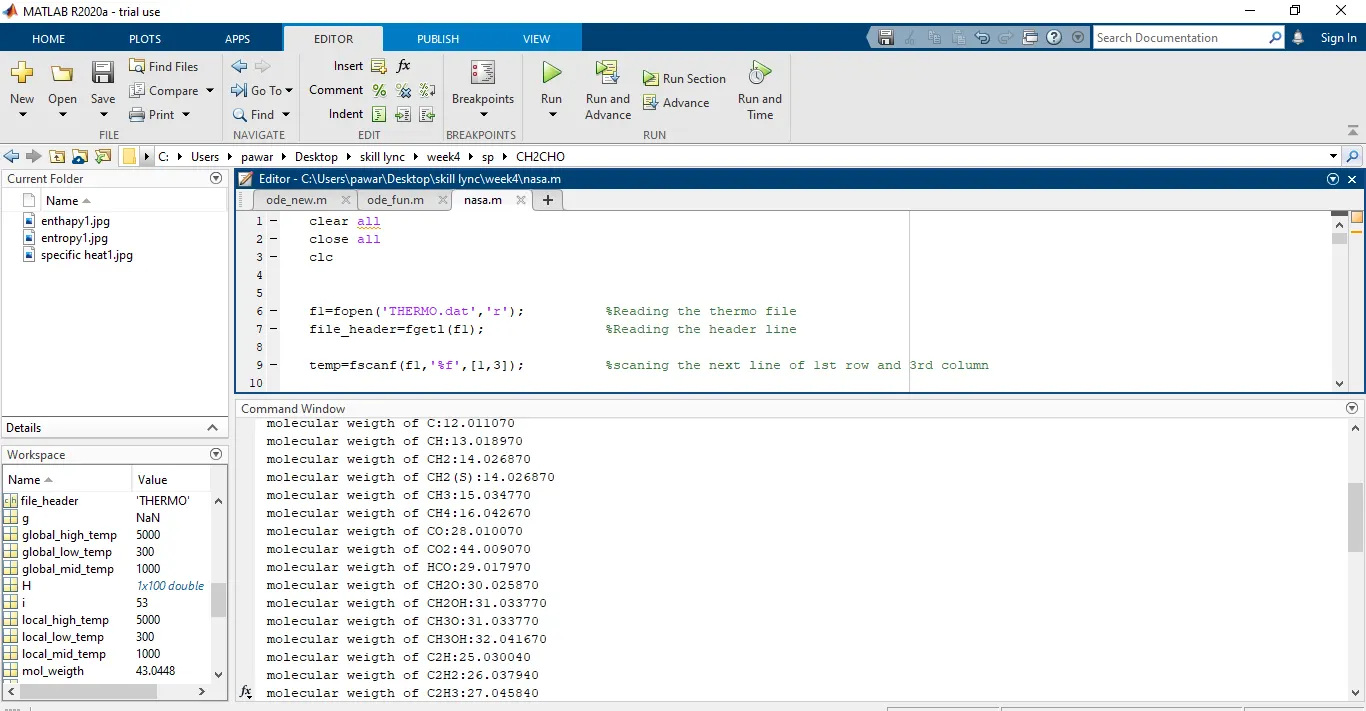
Calculated value of molecular weigth:

Conclusion:

Using MATLAB program data in the THERMO file is transformed into readeable content i.e into different graph of Specific heat, Enthalphy and Entrophy. MOlecular weigth of different species is also calculated.