WEEK 4 - Curve Fitting using MATLAB
AIM:
To write a code to perform curve fitting using MATLAB
Challenge expectation:
- Write a code to fit a linear and cubic polynomial for the Cp data provided.
- Plot the linear and cubic fit curves along with the raw data points.
- write a code to show the Split-wise method.
- Explain the parameters used to measure the fitness characteristics for both curves.
Questions asked:
- How to make a curve fit perfectly?
- How to get the best fit?
- What could be done to improve the cubic fit?
CONCEPT:
- Curve fitting is the process of constructing a curve or mathematical function, that has the best fit to a series of data points, possibly subject to constraint.
- There are many cases in that curve fitting can prove useful:
- quantify a general trend of the measured data.
- to remove noise from a function.
- extract meaningful parameters from the learning curve.
- summarize the relationships among two or more variables.
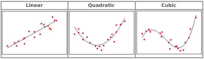
- For best fit, we assume that the measured data points are noisy. so, we don't want to fit a curve that intercepts every data point. Our goal is to learn a function that minimizes some predefined error on the given data points.
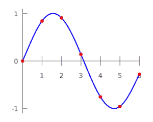
- For Exact fit, we assume that the given samples are not noisy, and we want to learn a curve that passes through each point. It is useful in cases we want to derive finite-difference approximations or to find minimums, maximums, and zero crossings of functions.
- Choosing the best fit depends upon finding a curve that satisfies that data points there are 4 quantities that helps us measure the goodness of fit criteria or how well the equation is representing the data points. They are :
1. The sum of squares due to error. (SSE)
2. R-square.
3. Adjusted R-square.
4. Root mean squared error. (RMSE) - The sum of square due to error (SSE)
Assume data points (x1,y1), (x2,y2), (x3,y3) ....(xn,yn) and assume the best fit for these set of points will be y=f(x) the criterion under which the equation of the curve will be the best fit possible as it follows,
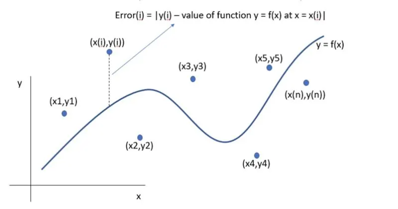
Suppose each of these n points has an individual error (difference in y co-ordinate values)
The error for the general T point can be given by the function,
To remove the modulus sign, it is effective if we squared the error term, when we square the error terms and add the errors for all the 'n' points we get,
When we differentiate the SSE with each and every coefficient of the proposed equation f(x) and equate it to zero, we can find the minima and the value of the coefficient.
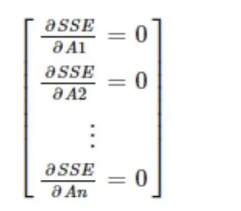
upon solving the multiples systems of equations we can find the values of all the coefficients.
This method is known as the Least Square Method and is the most commonly used technique as long as the fitting function is a polynomial. - R - square
This quantity measures how successful the fit is in explaining the variation of the data. Put another way, R-Square is the square of the correlation between the response values and the predicted response values. It is also called the square of the multiple correlation coefficient and the coefficient of multiple determination.
That is the higher the value of R-square the better the fit, the lower it is the lousier the fit, R-square ranges from a value of 0 to 10
* 0 for the worst possible fit for the data set.
* 1 for the best possible fit for the data set.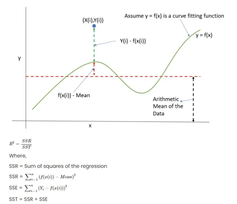
- Adjusted R-square
Adjusted R-square is a normalizing variation of R-square which neglects the variation of R-square due to insignificant independent variables.
* If the value of x(i) contributes to the output y, then x(i) is a significant dependent variable.
* If the value of x(i) does not contribute to the output y, then x(i) is an insignificant dependent variable.
Adjusted R-square disregards these infinitesimally small increments to R-square, and only considers the variables which actually contribute to the output of the systems in a drastic way.
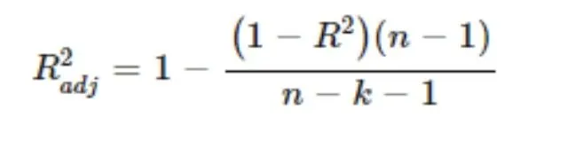
Where,
n = the number of data points.
k = the number of independent variables.
Here, there can be two possibilities:
1. The newly added independent variable is significant.
2. The newly added independent variable is insignificant. - Root mean square error (RMSE)
This statistic is also known as the fit standard error and the standard error of the regression. It is an estimate of the standard deviation of the random component in the data, and it is defined as,

Where n is the total number of data points available.
Using these four quantities in MATLAB effectively deduces the goodness of fit, typically if R-square is greater than 0.95 the fit is assumed to be good.
- Original Data set given:
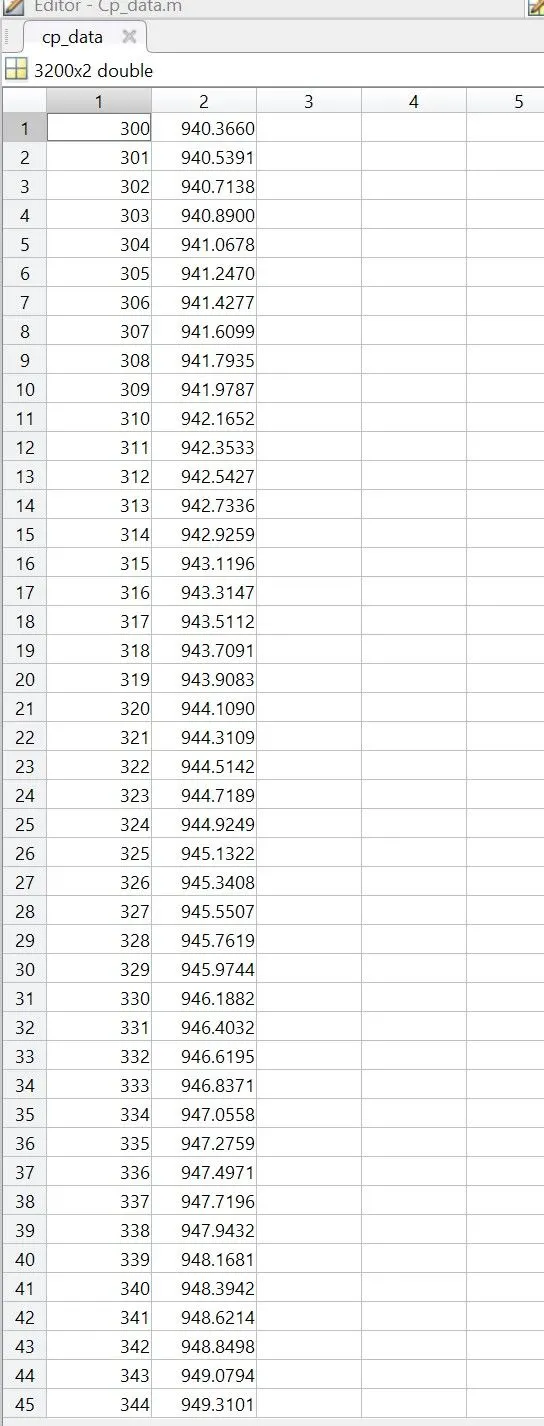
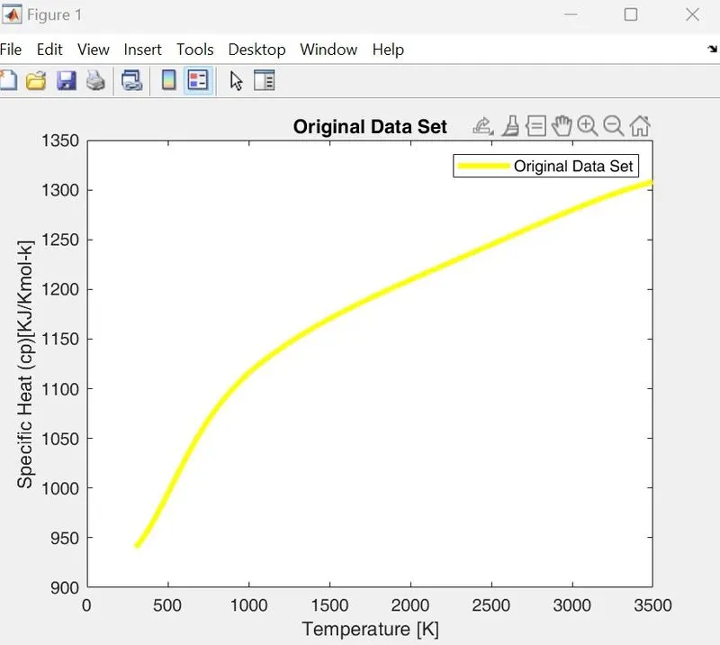
PROCEDURE:
clc
close all
clear all

% Loading the data file which has values od cp at various temperature
cp_data = load('data');
temperature = cp_data(:,1);
cp = cp_data(:,2);

% Curve Fitting
% For linear function which has a polynomial degree of 1 | cp = a*t+b
co_effs1 = polyfit(temperature,cp,1);
predicted_cp1 = polyval(co_effs1,temperature);

% For cubic function which has a polynomial degree of 3 | cp = a*t^3+b^2+ct+d
co_effs2 = polyfit(temperature,cp,3);
predicted_cp2 = polyval(co_effs2,temperature);

% Lets compare the original plot with linear curve fit
figure(1)
subplot(2,1,1)
% Plotting the original plot
hold on
plot(temperature,cp,'linewidth',3);
% Plotting the linear curve fit
plot(temperature,predicted_cp1,'linewidth',3,'color','r');
xlabel('Temperature [K]');
ylabel('Specific Heat (cp)[KJ/Kmol-k]');
legend('Original Data Set','Linear Curve Fit');
title('Linear Curve Fit');
hold off

% Now lets compare the original plot with our cubic curve fit
subplot(2,1,2)
% Plotting the original plot
hold on
plot(temperature,cp,'linewidth',3);
% Plotting of the cubic curve fit
plot(temperature,predicted_cp2,'linewidth',3,'color','c');
xlabel('Temperature [K]');
ylabel('Specific Heat (Cp) [KJ/Kmol-k]');
legend('Original Data Set','Cubic Curve Fit');
title('Cubic Curve Fit');
hold off

% Now lets compare all the plots (Original Plot, Linear Fit and Cubic Fit)
figure(2)
hold on
plot(temperature,cp,'linewidth',2);
plot(temperature,predicted_cp1,'linewidth',3,'color','r');
plot(temperature,predicted_cp2,'linewidth',3,'color','c');
xlabel('Temperature [K]');
ylabel('Specific Heat (Cp) [KJ/Kmol-k]');
legend('Original Data Set','Linear Curve Fit','Cubic Curve Fit');
title('Linear Fit vs Cubic Fit');
hold off

% Calculation for Best Fit

% Calculation of Sum of Squares due to Error (SSE)
SSE_L = sum((cp-predicted_cp1).^2);              % For Linear Fit
SSE_C = sum((cp-predicted_cp2).^2);              % For Cubic Fit

% Calculation of R-square
M = mean(cp);      % MEan for the R-square Calculation
% For Linear Fit
SSE_linear = sum((cp - predicted_cp1).^2);         % Sum of squared errors
SSR_linear = sum((predicted_cp1 - M).^2);        % Sum of square of regression

SST_linear = SSE_linear+SSR_linear;              % Total of sum of squares

% Calculating R-square for Linear fit
Rsquare_L = SSR_linear/SST_linear;

% For Cubic Fit
SSE_cubic = sum((cp-predicted_cp2).^2);          % Sum of squared errors
SSR_cubic = sum((predicted_cp2 - M).^2);         % Sum of squares of regression

SST_cubic = SSE_cubic+SSR_cubic;                 % Total of sum of squares

% Calculating R-Square for Cubic Fit
Rsquare_C = SSR_cubic/SST_cubic;

% Calculation of Adjusted R-Square
k = 1;
AdRsquare_L = 1- (((1-Rsquare_L)*(length(cp)-1))/(length(cp)-k-1));  % For Linear Fit
AdRsquare_C = 1- (((1-Rsquare_C)*(length(cp)-1))/(length(cp)-k-1));  % For Cubic Fit

% Calculation of Root Mean Squared Error (RMSE)
RMSE_L = sqrt(SSE_L/length(cp));                  % For Linear Fit
RMSE_C = sqrt(SSE_C/length(cp));                  % For Cubic Fit

% Putting Errors in the form of a Table
Name_of_Errors = {'SSE';'R_Square';'AdjustedR_Square';'RMSE'};

Linear_Fit_Error = [SSE_L; Rsquare_L; AdRsquare_L; RMSE_L];
Cubic_Fit_Error = [SSE_C; Rsquare_C; AdRsquare_C; RMSE_C];

disp('Best Fit Parameters for Linear and Cubic Curve Fit')
Best_Fit_Parameters = table(Linear_Fit_Error,Cubic_Fit_Error,'RowNames',Name_of_Errors)
CODE EXPLANATION:
clear all - To clear all the variables from the current workspace.
clc - Clear all the texts from the command window.
close all - Close all figures whose handles are visible.
linspace - The linspace function generates linearly spaced vectors.
plot - This command is used to Plot Graph.
Linewidth - The line width command is given to the width of the line which is going to be plotted on a graph.
xlabel - labeling X-axis.
ylabel - labeling Y-axis.
title - For giving title to the graph.
legend - It is used for indication of the line.
axis - For assigning axis to the plot.
RESULTS for Linear Fit and Cubic Fit Curve:
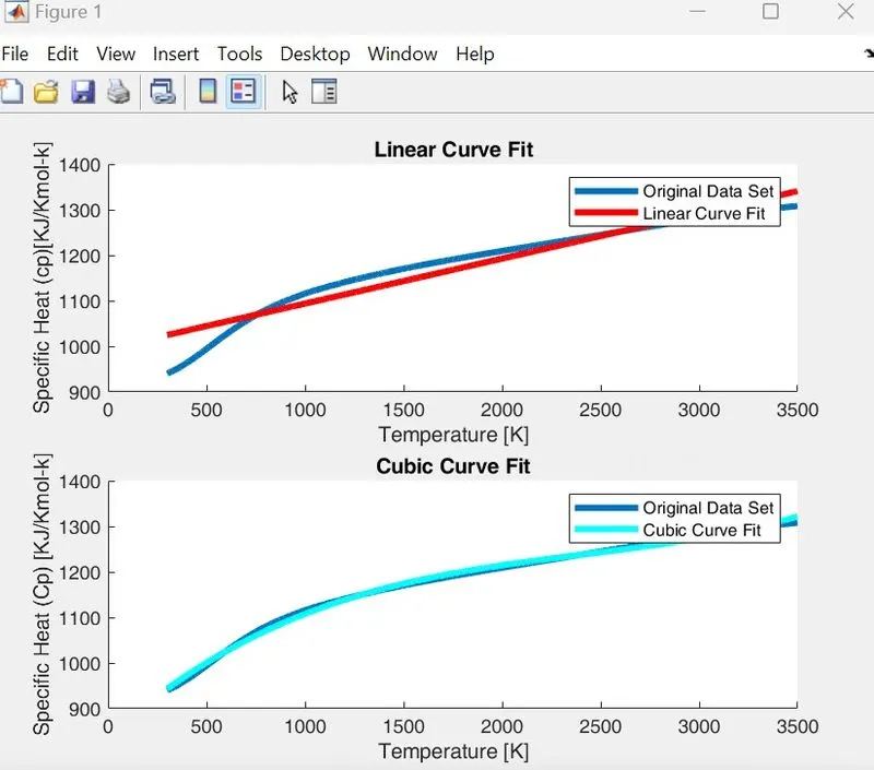
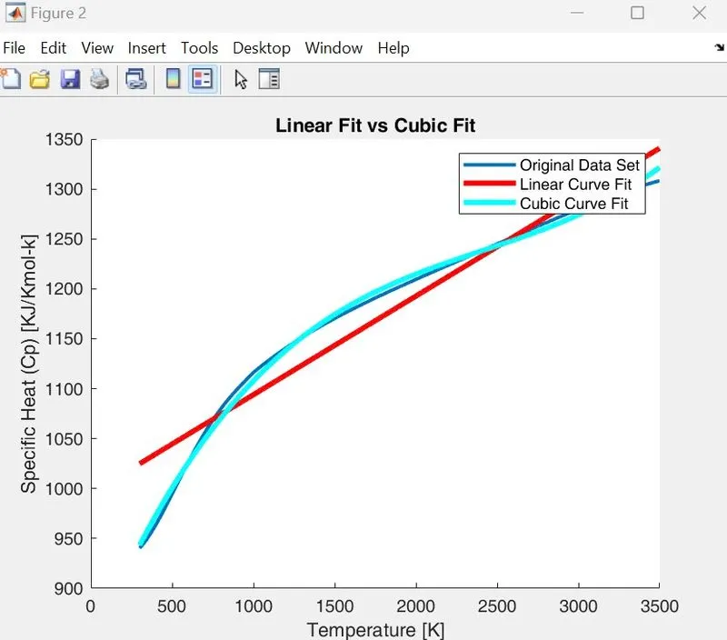
(A) (B)
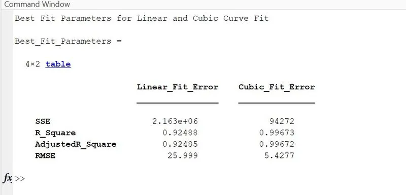
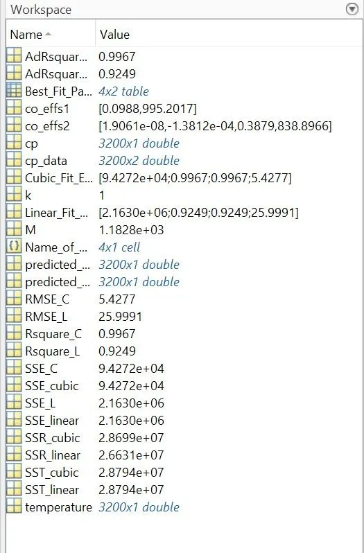
(C) (D)
ERRORS WHILE PROGRAMMING:
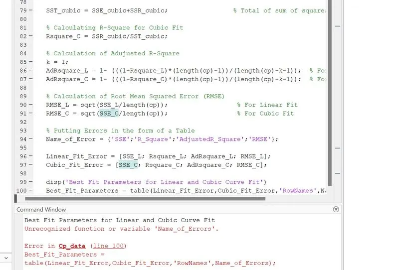
(A)
- Using the Curve fitting toolbox in MATLAB to validate our fitness characteristics.
1. For Linear Fit Curve.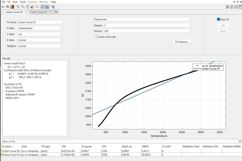
2. For Cubic Fit Curve.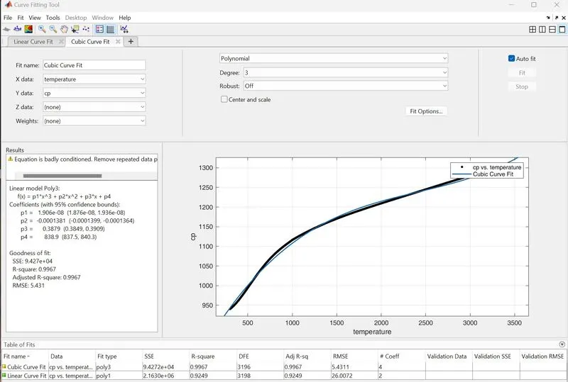
Split-Wise Code
clear all
close all
clc

% Loading the data file which has value of Cp at various temperature
cp_data = load('data')
temperature = cp_data(:,1);
cp = cp_data(:,2);

% Dividing Temperature and Specific Heat into 5 Parts
temperature_1 = cp_data(1:640,1);
predicted_cp_1 = cp_data(1:640,2);

temperature_2 = cp_data(641:1280,1);
predicted_cp_2 = cp_data(641:1280,2);

temperature_3 = cp_data(1281:1920,1);
predicted_cp_3 = cp_data(1281:1920,2);

temperature_4 = cp_data(1921:2560,1);
predicted_cp_4 = cp_data(1921:2560,2);

temperature_5 = cp_data(2561:3200,1);
predicted_cp_5 = cp_data(2561:3200,2);

% For Linear Polynomial | Cp = a*t+b
[co_efficient_lp, s1,mu1] = polyfit(temperature_1,predicted_cp_1,3);
predicted_specific_heat_1 = polyval(co_efficient_lp,temperature_1, s1,mu1);

% For Quadratic  Polynomial | Cp = a(t^2)+b(t)+c
[co_efficient_Qp, s2,mu2] = polyfit(temperature_2,predicted_cp_2,3);
predicted_specific_heat_2 = polyval(co_efficient_Qp,temperature_2, s2,mu2);

% For 3rd Degree Polynomial | Cp = a(t^3)+b(t^2)+c(t)+d
[co_efficient_3p, s3,mu3] = polyfit(temperature_3,predicted_cp_3,3);
predicted_specific_heat_3 = polyval(co_efficient_3p,temperature_3, s3,mu3);

% For 4th Degree Polynomial | Cp = a(t^4)+b(t^3)+c(t^2)+d(t)+e
[co_efficient_4p, s4,mu4] = polyfit(temperature_4,predicted_cp_4,3);
predicted_specific_heat_4 = polyval(co_efficient_4p,temperature_4, s4,mu4);

% For 5th Degree Polynomial | Cp = a(t^5)+b(t^4)+c(t^3)+d(t^2)+e(t)+f
[co_efficient_5p, s5,mu5] = polyfit(temperature_5,predicted_cp_5,3);
predicted_specific_heat_5 = polyval(co_efficient_5p,temperature_5, s5,mu5);

% Curve Fit Plot
figure(1)
plot(temperature,cp,'linewidth',2)
hold on
plot(temperature_1,predicted_specific_heat_1,'color','y','linewidth',3)
plot(temperature_2,predicted_specific_heat_2,'color','r','linewidth',3)
plot(temperature_3,predicted_specific_heat_3,'color','m','linewidth',3)
plot(temperature_4,predicted_specific_heat_4,'color','b','linewidth',3)
plot(temperature_5,predicted_specific_heat_5,'color','g','linewidth',3)
hold off
xlabel('Temperature [K]')
ylabel('Specific Heat [KJ/Kmol-k]')
title('Split Wise Curve Vs Original Curve Fit')
axis([250 3600 900 1400])
legend('Original Data','Linear Curve','Quadratic Curve','3rd Degree Curve ','4th Degree Curve','5th Degree Curve''location','best')
Code explanation:
plot - This command is used to Plot Graph.
Linewidth - The line width command is given to the width of the line which is going to be plotted on a graph.
title - For giving title to the graph.
legend - It is used for indication of the line.
axis - For assigning axis to the plot.
Results of Split-wise Program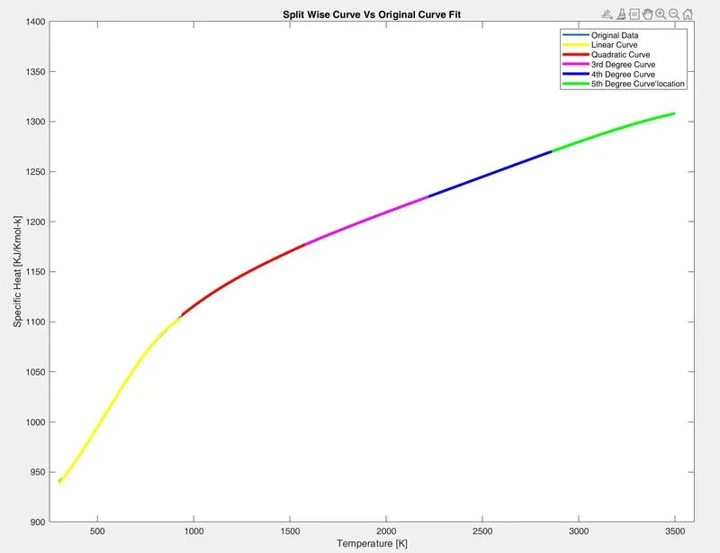
Error while coding split-wise code
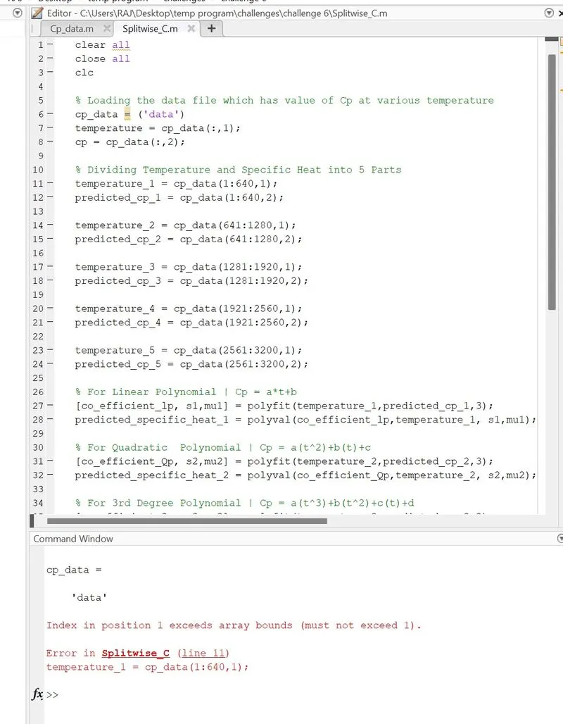
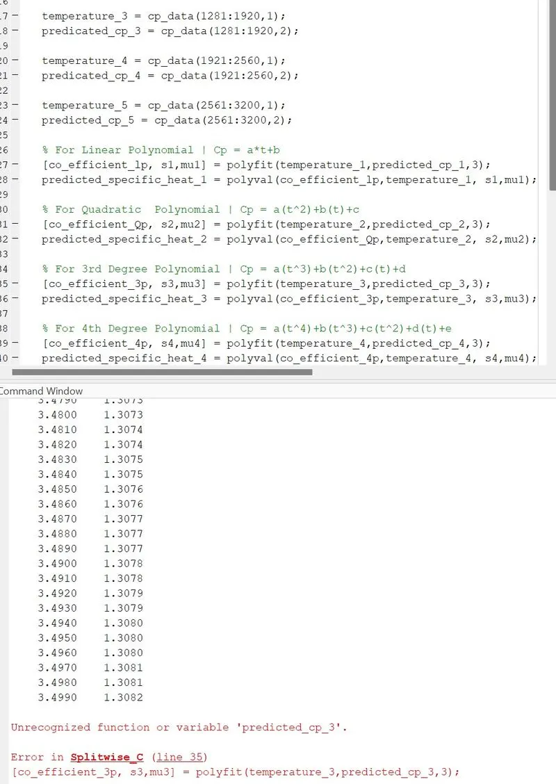
(A) (B)
REFERENCES:
- https://www.youtube.com/watch?v=0pqSL3ezwVo
- https://en.wikipedia.org/wiki/Curve_fitting
- https://in.mathworks.com/help/curvefit/index.html?s_tid=CRUX_lftnav
- https://skill-lync.com/student-projects/Curve-Fitting-and-criterion-to-choose-best-fit-41860
- https://www.youtube.com/watch?v=kXAtvLHJAus
Questions Asked:
1. How to make a curve fit perfectly?
The perfect fit means, the curve should fit the original curve without showing any errors in that particular degree of the polynomial. This means that every data point in the original plot should be on the curve. The perfect fit can always be the best fit but the best fit cannot be a perfect fit. We can fit a curve perfectly only by using interpolation. It is not necessary that we get a single function representing a complete trend.
2. How to get the best fit?
Best fit simply means that the differences between the actual measured Y values and the Y values predicted by the model equation are minimized. It does not mean a "perfect fit", in most cases, a least-squares best fit does not go through all the points in the data set. Above all, a least-squares fit must conform to the selected model.
We can get the best fit by:
1. Using higher degree polynomial.
2. Using split-wise curve fitting.
To compare the accuracy of fit, we can evaluate the goodness parameter. Once the improvement in the goodness parameter becomes stagnant, the best fit curve is obtained.
3. What could be done to improve the cubic fit?
To improve the cubic fit we can do the split-wise fitting for the curve. That is splitting the curve into multiple parts and using a different cubic polynomial for different sets of temperature and specific heat values. This reduces the errors and the best fit is obtained. Here I have split the data into five regions and performed a split fitting for the cubic function.