Week - 4 - Crash Box Simulation

Aim:

To simulate the crash test for the given crash box having a thickness of 1.2 and 1.5mm onto a rigid wall at 50kmph and to obtain the following output and data.

• Input .k file and output files (d3plot, glstat, sleout, rcforc)
• Animation of the final simulation
• The cross-sectional force generated in the middle of the crash box (along its length)
• Acceleration plot of a node in the middle of the crash box (along its length)
• Maximum directional stress and strain along the length of the crash box (X strain, Y strain, etc)
• The plot of all energies (total, internal, kinetic, hourglass, sliding)
• Compare the accelerations and stress/strain plots of 1.2/1.5mm crash boxes.

Theory:

The crash box is a thin-walled component which deforms axially and absorbs the energy during impact. The crash box is widely used in the automobile and aerospace industry to absorb accidental impact energy. So in the case of an automobile, the crash box is a separate component that is mounted in between the mainframe of the car and the front bumper. At the time of the accident, it deforms axially and absorbs accidental energy. Crash box structure provides comfort to the passenger at the time of impact. It works as a safeguard for the costly components behind the bumper like the engine hood and cooling system.

Procedure:

Import .k file, to import file>open>LS-DYNA keyword file. Figure1 shows the imported model. Figure2 shows the keywords used in the importd file.

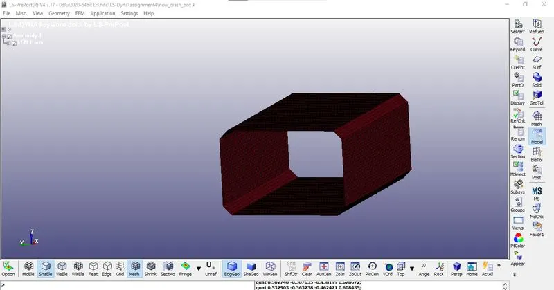Figure1

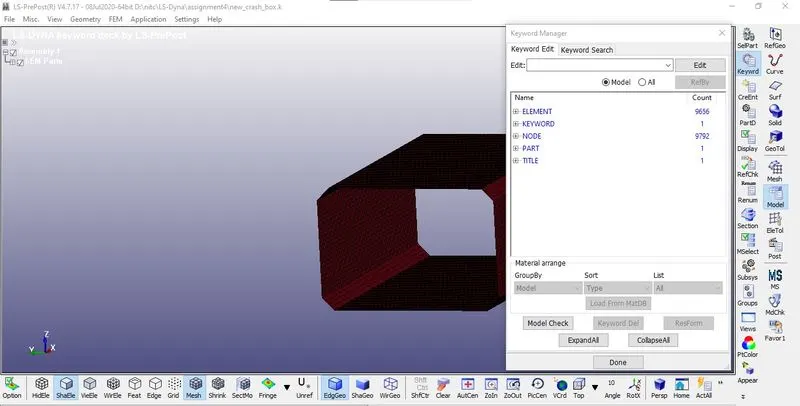Figure2

The unit system followed for the unit consistency is gm-mm-ms.

2. Create a Shell section card using the Model and Part > Keyword Manager > SECTION > Select the Shell option with Element formulation=2 and thickness = 1.2mm as shown in figure3

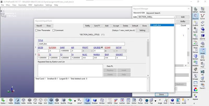Figure3

3. Define the material for the crash box component. Select the 024-PIECEWISE LINEAR PLASTICITY material card for the crash box component.

Model and Part> Keyword Manager > MAT > Select the Material card

Next, define the material properties like mass density, Young's modulus, Poisson's ration, Yield point stress value, and other required quantities for the material cards as shown in figure4.

• Density= 0.00783 `(gm)/(mm3)`
• Young's modulus 2.10 e+05 `(gm)/ (mm.ms2)`
• Poissions ratio=0.33
• Yield strength =310 `(gm)/(mm.ms2)`
• Tangent modulus = 2100 `(gm)/(mm.ms2)`

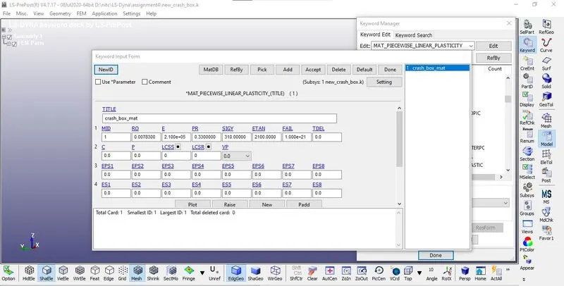
Figure4

4. Specifying the respective Material and Section ID to the crash box component part IDs as shown in Figure5

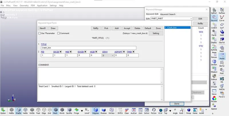Figure5

5. Next step is to create a Rigid wall in front of the crash box 10 mm away by using the "RIGIDWALL_PLANAR card

This is done by selecting Entity Creation > RigidWall Create as shown in Figure6. The rigid wall type is selected as a Planar and defined vector with one point and a normal ie, 1n+NL here selected the one node, and the normal is created as a rigid wall. This rigid wall is translated/offset by 10mm from the crash box component.

The black outer line shows the exact location of the rigid wall from the crash box component.

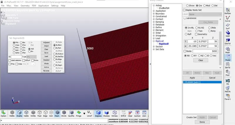Figure6

Note: The direction of normal (here x-direction) from the rigid wall and the velocity vector (x-direction) should be in the opposite direction in order to avoid the penetration of the crash box through the rigid wall which is not acceptable since it is a rigid wall and the component is a material which shows the plasticity.

6. Next step is to define a velocity of 50kmph (13.8889 mm/ms) and assigned to each node of the selected crash box component, under Entity Creation >Initial>Velocity>Insert the value. The Crash box is selected by pick option with respect to part as shown below figure7.

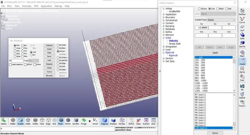Figure7

7. Create a Contact using Model and Part > Keyword Manager > Contact > Automatic Single Surface. The slave segment type (SSTYP) is defined by the Part ID, here there is no need to define a master surface so only the slave surface definition is sufficient as shown Figure8

After the automatic contact was created as the crash box elements are getting self contact during crashing ie, Automatic single surface here it was not needed to define the master surface because the crash box itself is master and slave.

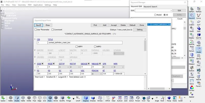Figure8

8. Next the Termination time is to be assigned by using *CONTROL_TERMINATION card. Here the time to end the simulation can be calculated analytically by using the distance between the rigid wall and crash box component ie,10mm, and the velocity of the crash box ie,13.8889 mm/ms.

End time, t = (10mm)/(13.8889 mm/ms) = 0.7199

The calculated time is 0.7199ms but extra time is considered after the impact in simulation ie, the crashing and the bouncing back of the crash box. So, the total time of Ims is assigned as end time in the "CONTROL_TERMINATION card as shown in Figure9

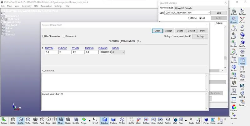Figure9

calculate the energy dissipation, Hourglass energy, rigid wall energy, sliding interface energy that can be done

by "CONTROL_ENERGY card as shown in Figure10

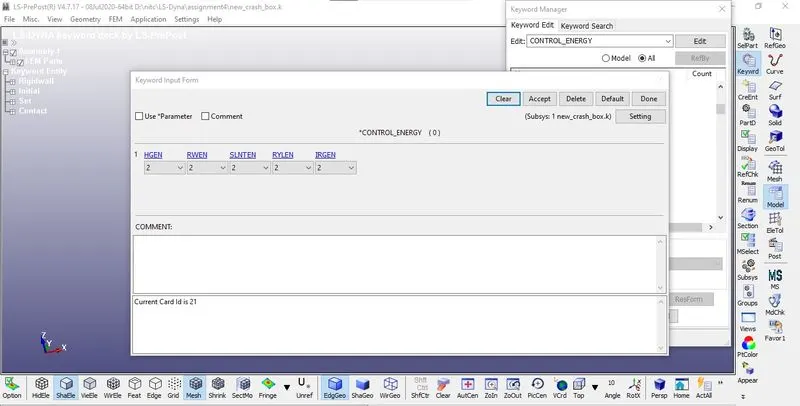Figure10

Finally create a "CONTROL_HOURGLASS card for control hourglass effect in the analysis with 1HQ=2, QH=0.1 as shown in Figure11.

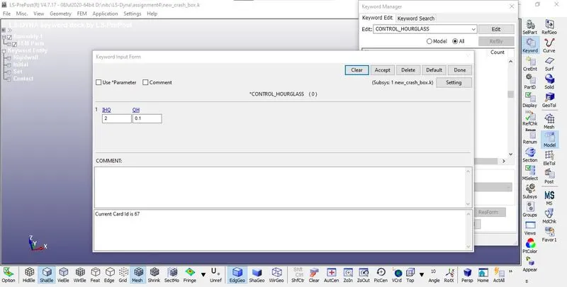Figure11

9. Now, the following output data is generated by using the "DATABASE card with a time step of 0.01ms are assigned for generating output data as shown in Figure12&13.

DATABASE_BINARY_D3PLOT--> Used to find out the animation of the process,

DATABASE ASCII_NODOUT--> To find the Nodal motions,

DATABASE_ASCII_ELOUT --> To find the element data,

DATABASE_ASCII GLSTAT To find the global statistics and energies,

DATABASE_ASCII_MATSUM --> To find the material energies,

DATABASE ASCII_RCFORC--> To find the Resultant contact interface forces,

DATABASE ASCII_SLEOUT--> To find the Contact interface energies

DATABASE ASCII_SECFORC To find the Cross-section forces data

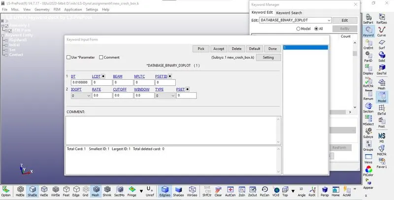Figure12

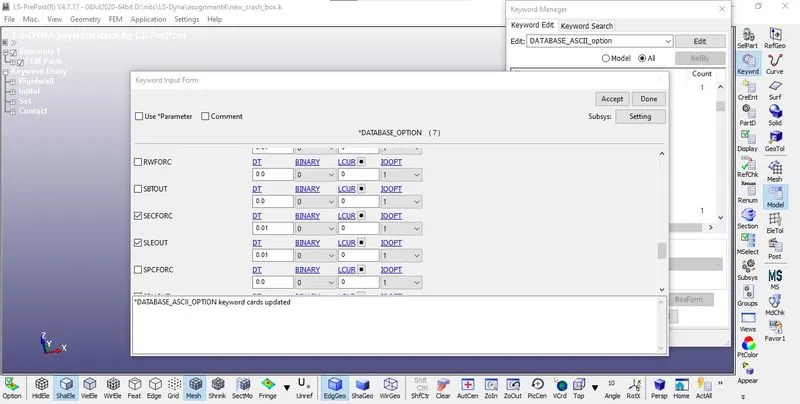Figure13

For generating section forces creating a specific node and element/shell list which defines the desired section of component is necessary. The selection of nodes and elements/shell lists is done by picking each node and element through Creating Entity>Set Data> *SET_NODE for node-set and Creating Entity>Set Data>"SET_SHELL for element/shell-set as shown in Figure14&15.

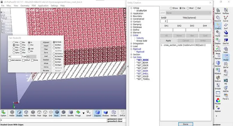Figure14

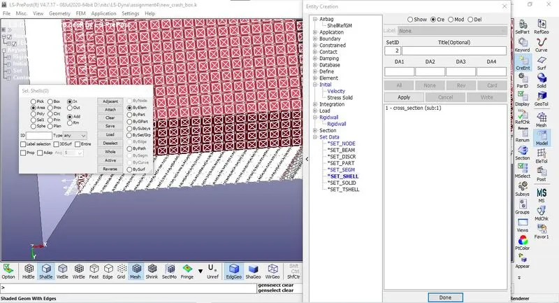Figure15

*DATABASE_CROSS_SECTION_SET card is used so as get nodes and element/shell set from the component and are assigned for node-set ID (NSID) and shell element set ID (SSID) respectively as shown in Figure16

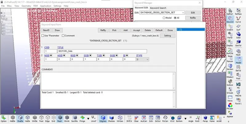Figure16

The acceleration plot of a node and element of the crash box can be done by picking the desired node and element by using "DATABASE_HISTORY_NODE and *DATABASE_HISTORY_SHELL card as shown in Figure17&18

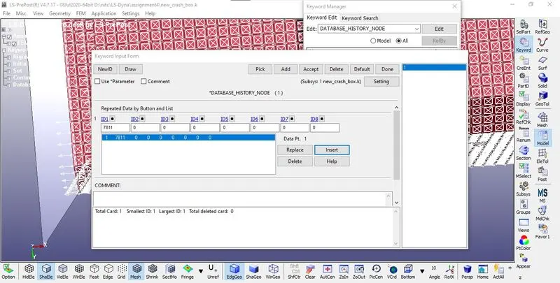Figure17

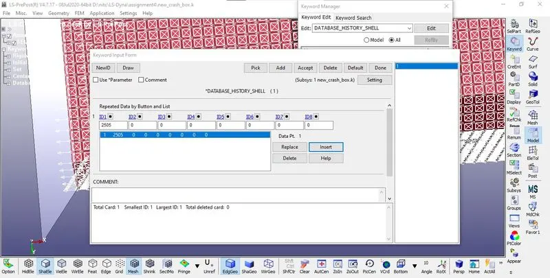Figure18

Model Checks:

check the model whether any errors were there and correct them.

Figure19 shows the model after correcting the errors.

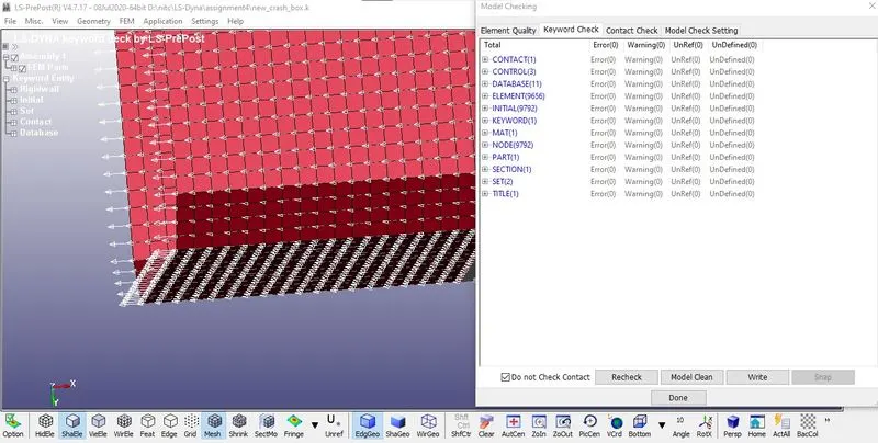Figure19

10. After assigning all the above-mentioned keywords, the model is ready for the simulation. The keyword file (.k) can be edited again so that the comparison study can be done for the part which is having 1.2mm and 1.5mm thickness. Save the keyword for both files and open in the LS-DYNA manager which solves the problem

RESULTS:

The Cross-sectional force generated in the middle of the crashbox (along its length) as shown in below for both 1.2mm and 1.5mm thickness

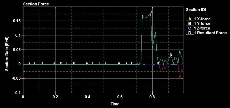
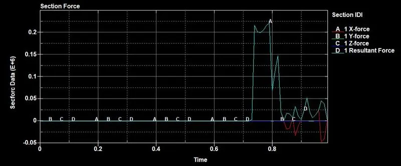
Note: From the above figure we can able to see that the force value at the Y and Z direction after impact is very low since the velocity value is in the X-direction. At the impact time, we can see that the force value in X-direction peaks up and goes down after bounce-back of the crash box. The Resultant force of a 1.5 mm thickness crash box is higher than that of a 1.2 mm thickness crash box since as per Newton's second law we know that F=ma, here 1.5 mm thickness crash box is having higher mass compared to the 1.2 mm thickness crash box and here the acceleration is same in both the case.

The Acceleration plot of a node in the middle of the crashbox (along its length) as shown in below figures for both 1.2mm and 1.5mm thickness

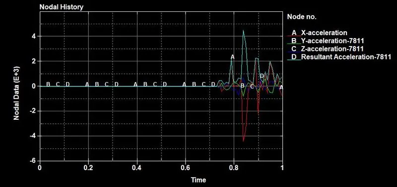
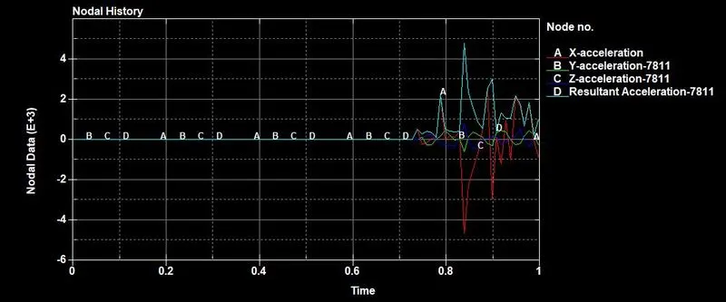
Note: From the above figure 15(a) & 15(b) we can able to see that the nodal acceleration in the X-direction is negative since the accelerated body when came to impact there a deceleration happened. Here the value of deceleration in X-direction is nearly the same and the resultant acceleration is a magnitude and doesn't depend on the direction so we can see the positive value and almost equals the value of X-direction magnitude since the acceleration value in the Y and Z direction is very small.

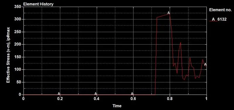
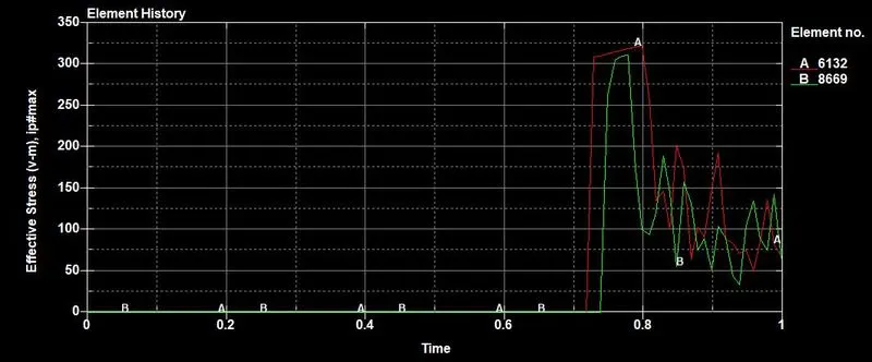
Stress plots are shown in below for both 1.2mm and 1.5mm thickness

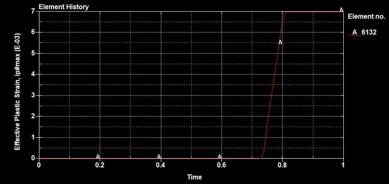
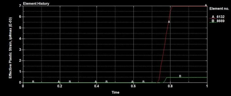
Strain plots are shown in below for both 1.2mm and 1.5mm thickness

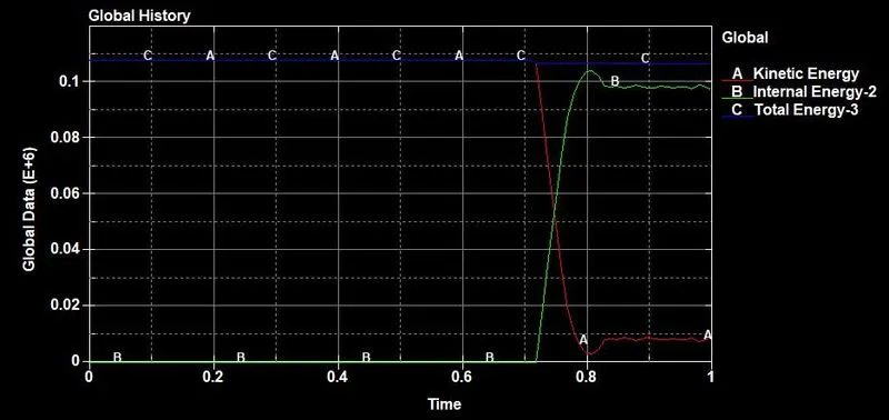
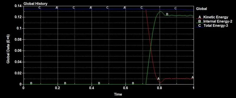
Energy plots are shown in below for both 1.2mm and 1.5mm thickness