Assignment 4-RADIOSS Material Laws Challenge

OBJECTIVE : Compare the results obtained by simulating different cases Material Laws and plot their results.

PROCEDURE :

CASE1 : Run the model as it is without chaning any previous values in FAILURE_JOHNSON file.

- Import FAILURE_JOHNSON_0000.rad file by going into the import section as shown in Figure1

- After importing the model will be look like as shown in Figure 2

- Change wire frame of the model into the solid frame as shown in Figure 3

- Look into the properties of the Material given already as shown in Figure 4&5

- To run the simulation Go to analysis section select Radioss, in which select where to save the file and name of the file Law2_epsmax_failure_000.rad and choose -nt 4 in options, it means run four cpus at a time to run the simulation faster and run the simulation as shown in Figure 6

- After completion of simulation Altair Compute Console Solver View tab will be appear as shown in Figure 7, in which we can came to know whether our simulates successfully or not, any errors and warnings will be shown there if simulation stops in between.

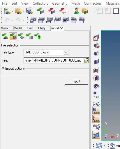
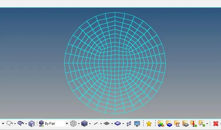
Figure 1 Figure 2

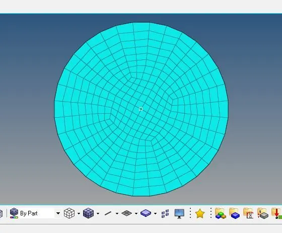
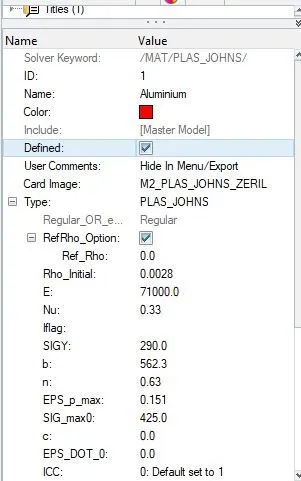
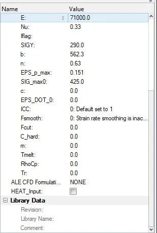
Figure 3 Figure 4 Figure 5

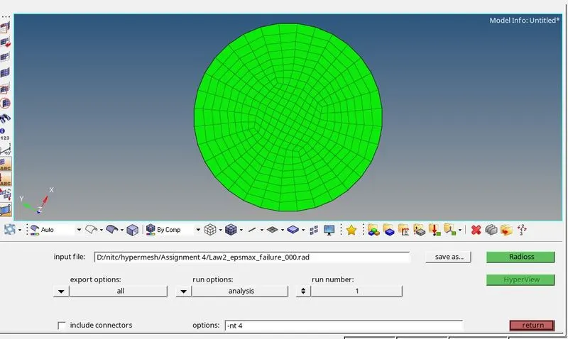
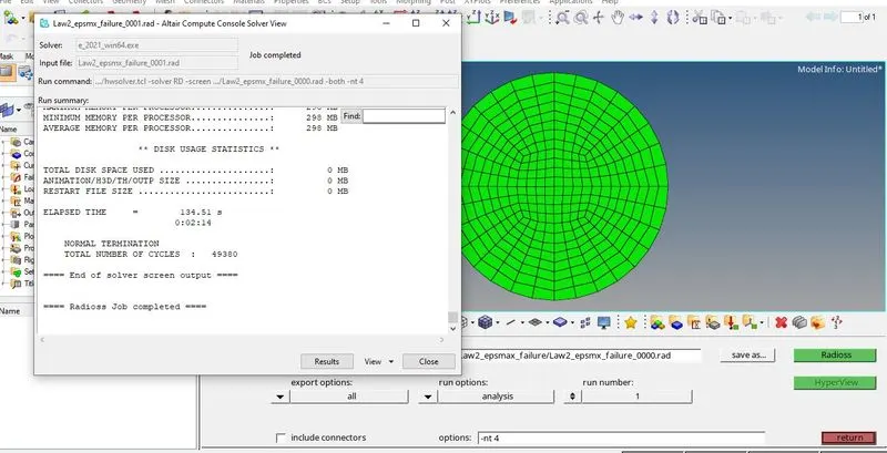
Figure 6 Figure 7

- After open the Law2_epsmax_failure_ooo1.out file in note pad and various values of Energy error, mass error are get as shown in Figure 8

1) Energy error -0.8%

2) Mass Error - 0.000

3) Number of cycles - 49380

4) Starter run time - 13.14s (00:00:13)

engine run time - 134.51s (00:02:14)

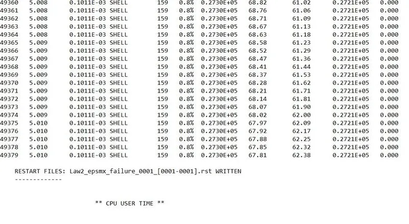Figure 8

- To look into the Animation files, Hyperview and in which .h3d file as given as a input and enter into the contour section in which selected Von-mises as a result type and remaining kept as a default and click on apply, we will animated file with max and minimum stresses developed in the model as shown in Figure 9 and Anmimated file is shown in video name as Law2_epsmax_failure.

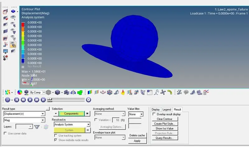Figure 9

- For Post processsing results entered into the HyperGraph 2D in which .T01 file is given as a inputs and various plots Rigidwall Force, kinetic energy, total energy, contact energy, hourglass energy are plotted as shown in Figure 10 &11.

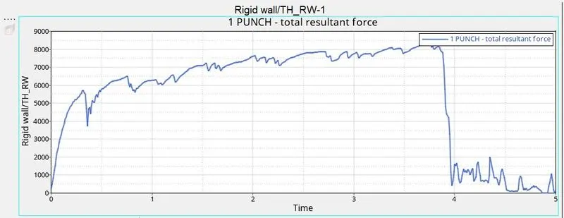Figure 10

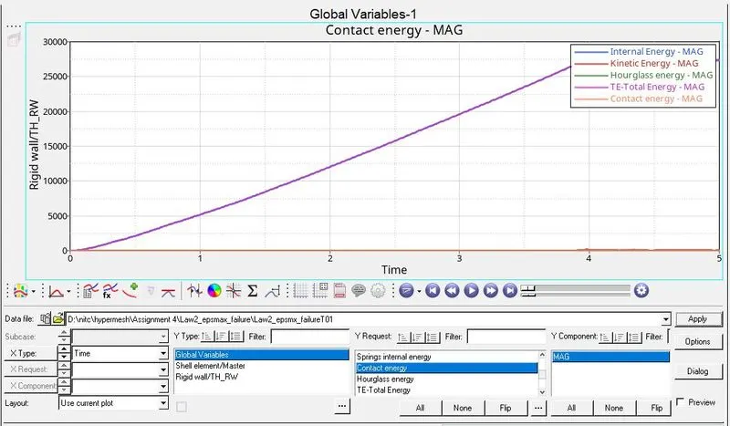Figure 11

CAESE 2 : IN/FAIL/JOHNSON, change Ifail_sh = 1, Dadv = 1, and ixtem=1 and run the model as Law2_epsmac_crack.

- Import FAILURE_JOHNSON_0000.rad file by going into the import section as shown in Figure 1.

- After importing the model will be look like as shown in Figure 2

- Change wire frame of the model into the solid frame as shown in Figure 3

- Look into the FAILURES section in the MODEL Browser and changed the values according to the question as Ifail_sh = 1, Dadv = 1, and ixtem=1 it is shown in Figure 12 & 13.

- To run the simulation Go to analysis section select Radioss, in which select where to save the file and name of the file Law2_epsmax_crack_000.rad and choose -nt 4 in options, it means run four cpus at a time to run the simulation faster and run the simulation.

- After completion of simulation Altair Compute Console Solver View tab will be appear in which we can came to know whether our simulates successfully or not, any errors and warnings will be shown there if simulation stops in between.

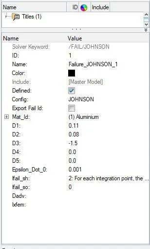Figure 12 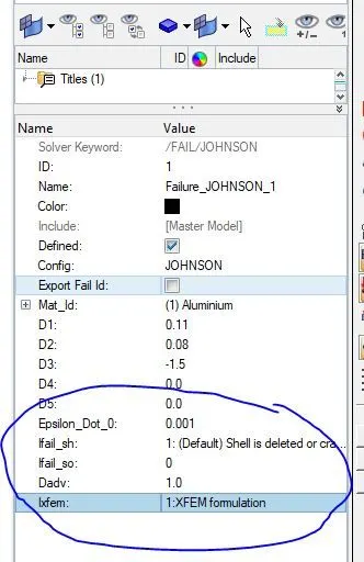Figure 13

- After open the Law2_epsmax_crack_ooo1.out file in note pad and various values of Energy error, mass error are get as shown in Figure 14

1) Energy error -4.1%

2) Mass Error - 0.000

3) Number of cycles - 49217

4) Starter run time - 14.96s (00:00:14)

engine run time - 191.12s (00:03:11)

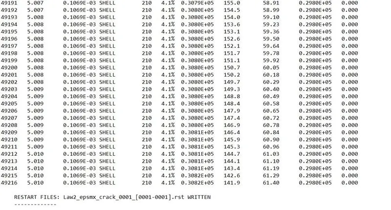Figure 14

- To look into the Animation files, Hyperview and in which .h3d file as given as a input and enter into the contour section in which selected Von-mises as a result type and remaining kept as a default and click on apply, we will animated file with max and minimum stresses developed in the model and Anmimated file is shown in video name as Law2_epsmax_crack.

- For Post processsing results entered into the HyperGraph 2D in which .T01 file is given as a inputs and various plots Rigidwall Force, kinetic energy, total energy, contact energy, hourglass energy are plotted as shown in Figure 15&16.

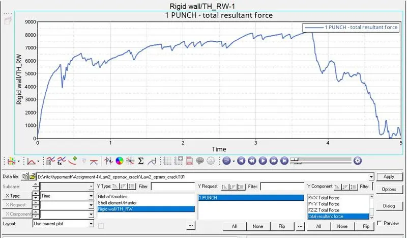Figure 15

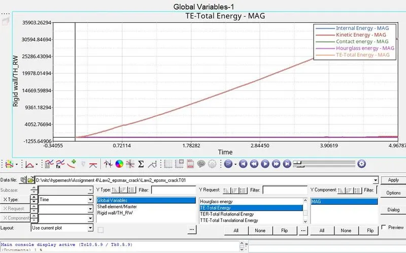Figure 16

CASE3: Delete /FAIL/JOHNSON card and run the file as Law2_epsmax_nofail

- Import FAILURE_JOHNSON_0000.rad file by going into the import section as shown in Figure 1.

- After importing the model will be look like as shown in Figure 2

- Change wire frame of the model into the solid frame as shown in Figure 3

- Look into the FAILURES section in the MODEL Browser and right click on that and delete the failure section as shown in figure 17.

- To run the simulation Go to analysis section select Radioss, in which select where to save the file and name of the file Law2_epsmax_nofail_000.rad and choose -nt 4 in options, it means run four cpus at a time to run the simulation faster and run the simulation.

- After completion of simulation Altair Compute Console Solver View tab will be appear in which we can came to know whether our simulates successfully or not, any errors and warnings will be shown there if simulation stops in between.

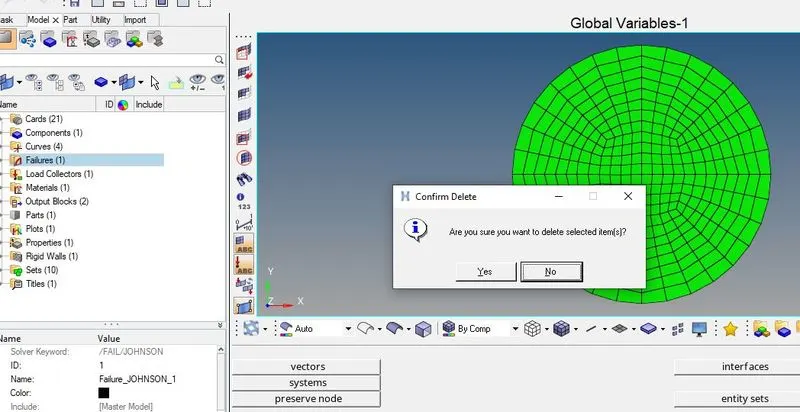Figure 17

- After open the Law2_epsmax_nofail_ooo1.out file in note pad and various values of Energy error, mass error are get as shown in Figure 18

1) Energy error - 0.8%

2) Mass Error - 0.000

3) Number of cycles - 49408

4) Starter run time - 6.12s (00:00:06)

engine run time - 151.81s (00:02:31)

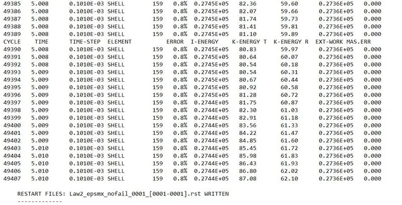Figure 18

- To look into the Animation files, Hyperview and in which .h3d file as given as a input and enter into the contour section in which selected Von-mises as a result type and remaining kept as a default and click on apply, we will animated file with max and minimum stresses developed in the model and Anmimated file is shown in video name as Law2_epsmax_nofail.

- For Post processsing results entered into the HyperGraph 2D in which .T01 file is given as a inputs and various plots Rigidwall Force, kinetic energy, total energy, contact energy, hourglass energy are plotted as shown in Figure 19&20.

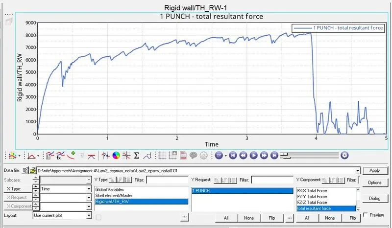Figure 19

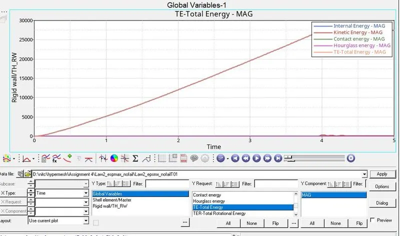Figure 20

CASE4: Delete the value of EPS_P_max and run the model with name Law2

- Import FAILURE_JOHNSON_0000.rad file by going into the import section as shown in Figure 1.

- After importing the model will be look like as shown in Figure 2

- Change wire frame of the model into the solid frame as shown in Figure 3

- Look into the MATERIALS section in the MODEL Browser and edit the value of EPS_P_max value as shown in Figure 21&22.

- To run the simulation Go to analysis section select Radioss, in which select where to save the file and name of the file Law2_000.rad and choose -nt 4 in options, it means run four cpus at a time to run the simulation faster and run the simulation.

- After completion of simulation Altair Compute Console Solver View tab will be appear in which we can came to know whether our simulates successfully or not, any errors and warnings will be shown there if simulation stops in between.

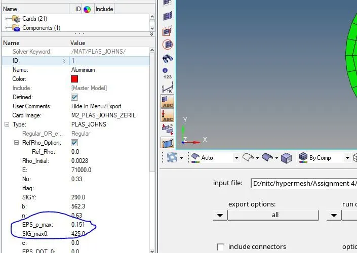
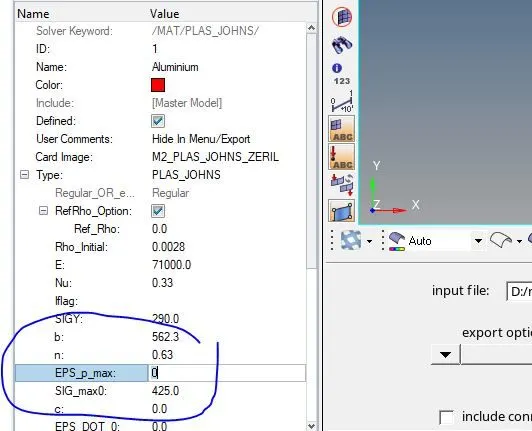
Figure 21 Figure 22

- After open the Law2_ooo1.out file in notepad and various values of Energy error, mass error are get as shown in Figure 23

1) Energy error - 1.1%

2) Mass Error - 0.000

3) Number of cycles - 49304

4) Starter run time - 1.67s (00:00:01)

engine run time - 177.18s (00:02:57)

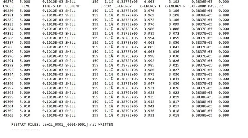Figure 23

- To look into the Animation files, Hyperview and in which .h3d file as given as a input and enter into the contour section in which selected Von-mises as a result type and remaining kept as a default and click on apply, we will animated file with max and minimum stresses developed in the model and Anmimated file is shown in video name as Law2.

- For Post processsing results entered into the HyperGraph 2D in which .T01 file is given as a inputs and various plots Rigidwall Force, kinetic energy, total energy, contact energy, hourglass energy are plotted as shown in Figure 24&25.

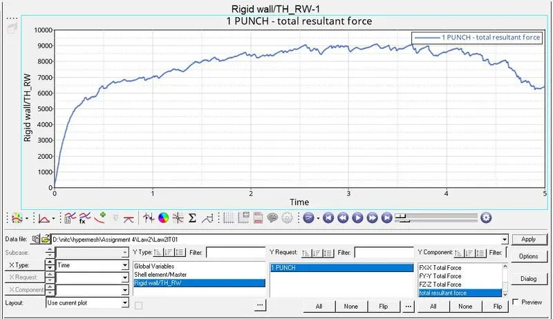Figure 24

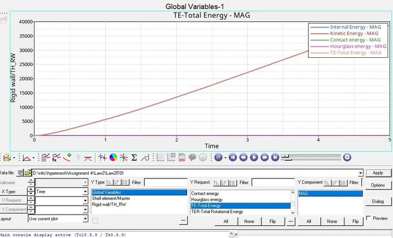Figure 25

CASE5: Convert the material model into Law1 elastic with same density, E, nu and run and checc the results.

- Import FAILURE_JOHNSON_0000.rad file by going into the import section as shown in Figure 1.

- After importing the model will be look like as shown in Figure 2

- Change wire frame of the model into the solid frame as shown in Figure 3

- Look into the MATERIALS section in the MODEL Browser and edit the material card value to 1 without changing E,nu values as shown in Figure 26&27.

- To run the simulation Go to analysis section select Radioss, in which select where to save the file and name of the file Law1_000.rad and choose -nt 4 in options, it means run four cpus at a time to run the simulation faster and run the simulation.

- After completion of simulation Altair Compute Console Solver View tab will be appear in which we can came to know whether our simulates successfully or not, any errors and warnings will be shown there if simulation stops in between.

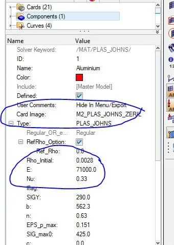Figure 26 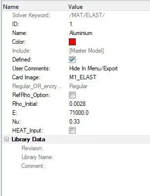Figure 27

- After open the Law1_ooo1.out file in notepad and various values of Energy error, mass error are get as shown in Figure 28

1) Energy error - 1.3%

2) Mass Error - 0.000

3) Number of cycles - 47969

4) Starter run time - 2.49s (00:00:02)

engine run time - 99.72s (00:01:39)

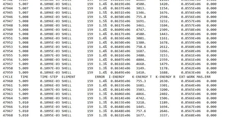Figure 28

- To look into the Animation files, Hyperview and in which .h3d file as given as a input and enter into the contour section in which selected Von-mises as a result type and remaining kept as a default and click on apply, we will animated file with max and minimum stresses developed in the model and Anmimated file is shown in video name as Law1.

- For Post processsing results entered into the HyperGraph 2D in which .T01 file is given as a inputs and various plots Rigidwall Force, kinetic energy, total energy, contact energy, hourglass energy are plotted as shown in Figure 29&30.

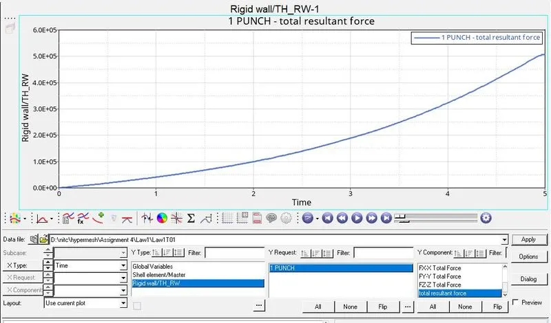Figure 29

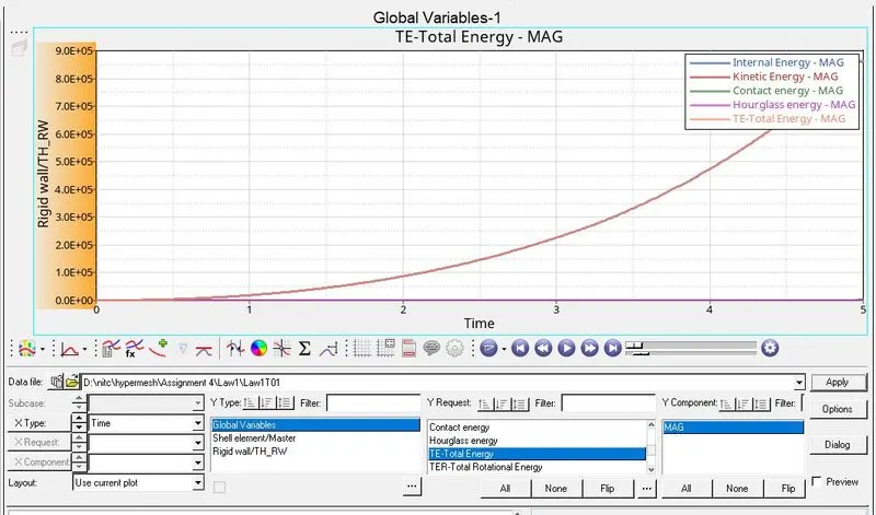Figure 30

CASE6: Open Law27 model file, change the shell properties to required shell properties and run the model as Law27

- Import Law27_0000.rad file by going into the import section.

- Change wire frame of the model into the solid frame.

- Look into the PROPERTIES section in the MODEL Browser and edit the required properties values as shown in Figure 31&32.

- To run the simulation Go to analysis section select Radioss, in which select where to save the file and name of the file Law27_000.rad and choose -nt 4 in options, it means run four cpus at a time to run the simulation faster and run the simulation.

- After completion of simulation Altair Compute Console Solver View tab will be appear in which we can came to know whether our simulates successfully or not, any errors and warnings will be shown there if simulation stops in between.

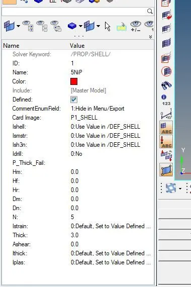Figure 31 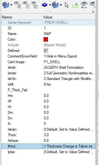Figure 32

- After open the Law27_ooo1.out file in notepad and various values of Energy error, mass error are get as shown in Figure 33

1) Energy error - 0.6%

2) Mass Error - 0.000

3) Number of cycles - 49486

4) Starter run time - 8.39s (00:00:08)

engine run time - 142.11s (00:02:22)

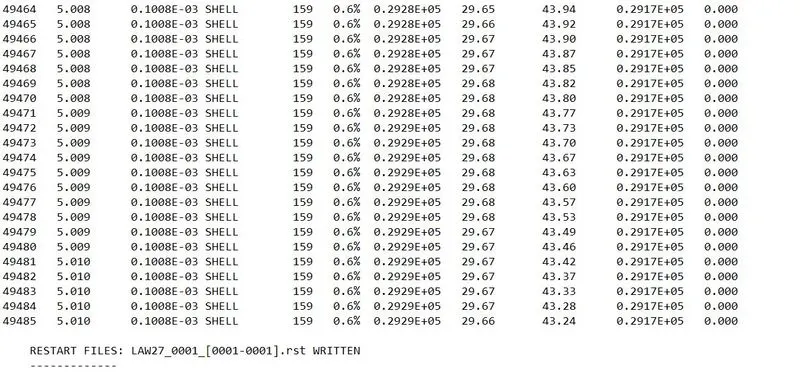Figure 33

- To look into the Animation files, Hyperview and in which .h3d file as given as a input and enter into the contour section in which selected Von-mises as a result type and remaining kept as a default and click on apply, we will animated file with max and minimum stresses developed in the model and Anmimated file is shown in video name as Law27.

- For Post processsing results entered into the HyperGraph 2D in which .T01 file is given as a inputs and various plots Rigidwall Force, kinetic energy, total energy, contact energy, hourglass energy are plotted as shown in Figure 34&35.

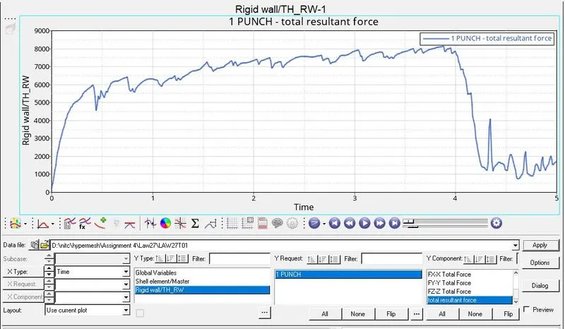Figure 34

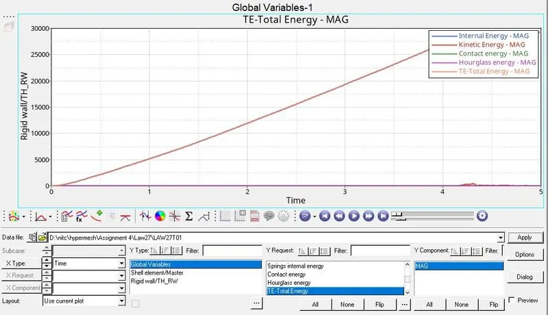Figure 35

CASE7: Create a Law36 material and change the shell properties to the required shell properties.

- Import Law27_0000.rad file by going into the import section.

- Change wire frame of the model into the solid frame.

- Look into the PROPERTIES section in the MODEL Browser and edit the required properties values as shown in Figure 36.

- Look into the MATERIALS section in the MODEL browser and change the material card to Law36 and change other parameters according to the video lecture that sir discussed in class is shown in figure 37&38, in between add curve as a one parameter to Material Law36 which is shown in Figure 39.

- To run the simulation Go to analysis section select Radioss, in which select where to save the file and name of the file Law36_000.rad and choose -nt 4 in options, it means run four cpus at a time to run the simulation faster and run the simulation.

- After completion of simulation Altair Compute Console Solver View tab will be appear in which we can came to know whether our simulates successfully or not, any errors and warnings will be shown there if simulation stops in between.

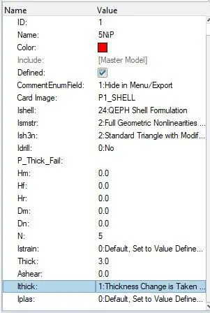Figure 36 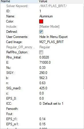Figure 37 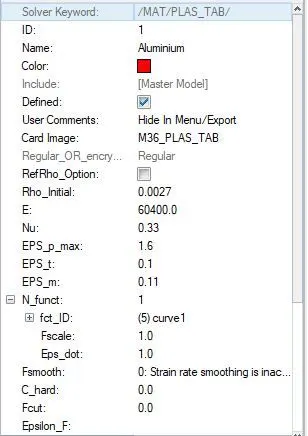Figure 38

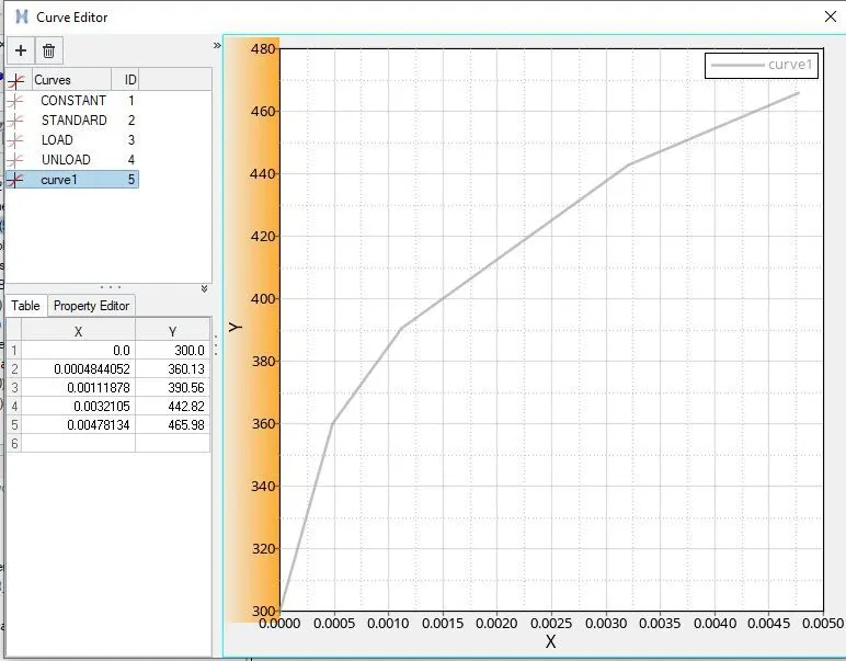Figure 39

- After open the Law36_ooo1.out file in notepad and various values of Energy error, mass error are get as shown in Figure 40

1) Energy error - 0.2%

2) Mass Error - 0.000

3) Number of cycles - 49044

4) Starter run time - 3.14s (00:00:03)

engine run time - 114.97s (00:01:54)

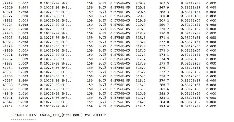Figure 40

- To look into the Animation files, Hyperview and in which .h3d file as given as a input and enter into the contour section in which selected Von-mises as a result type and remaining kept as a default and click on apply, we will animated file with max and minimum stresses developed in the model and Anmimated file is shown in video name as Law36.

- For Post processsing results entered into the HyperGraph 2D in which .T01 file is given as a inputs and various plots Rigidwall Force, kinetic energy, total energy, contact energy, hourglass energy are plotted as shown in Figure 41&42.

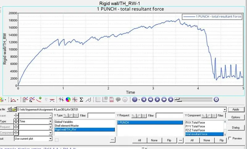Figure 41

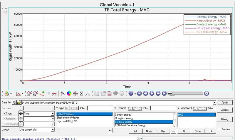Figure 42

COMPARISON OF THE 7 CASES:

CASES Energy error Mass error Total no of cycles Element deletion Material Laws used

case1 0.8% 0.00 49380 Element will be deleted Law2 with a,b,n values

case2 4.1% 0.00 49217 Element will be deleted Law2 by changing the values in Failures

case3 0.8% 0.00 49408 Element will be deleted Law2 by deleting Failure

case4 1.1% 0.00 49304 Element will be deleted Law2 by deleting EPS_max value

case5 1.3% 0.00 47969 Element will not deleted Law1

(purely elastic)

case6 0.6% 0.00 49486 Element will be deleted Law27

( Elasic-plastic brittle)

case7 0.2% 0.00 49044 Element will be deleted Law36

(Elasto plastic)

CONCLUSION:

There are so many laws indicated but for which material to fix which law is known by simulating to accurate result.