Crash Box Simulation in LS-Dyna

Objective: To simulate a crash test for a crash box with 1.2 and 1.5mm thickness using LS-Dyna.

Procedure:

• Open the supplied .k file, which contains the mesh information of the crash box.

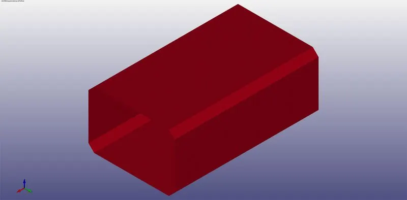
Fig 1: Mesh information of the crash box.

• The initial keyword file contains only the element, node, and parts information available within it. To fully develop the deck file to simulate the crash test, necessary keyword cards must be added to the model.

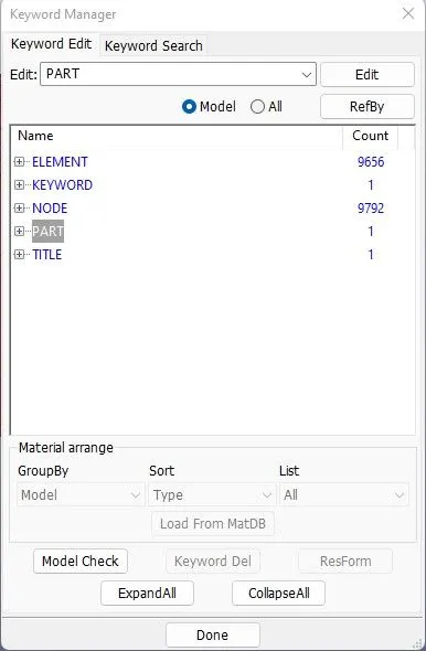
Fig 2: Initial keyword file information.

• To start with the deck preparation, we rename the auto-created parts with a suitable name and part ID to distinguish them and for further use.

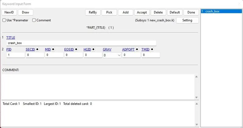
Fig 3: Rename the parts and IDs to differentiate them.

• A shell section keyword is included with shell element formulation(ELFORM=2) and assigning a thickness of 1.2mm. For the second simulation, only the thickness value in the section keyword is changed to 1.5mm, and the rest all remain the same.

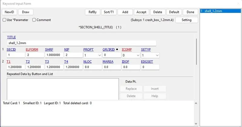
Fig 4: Element formulation is defined for the shell elements with 1.2mm thickness.

• MAT024-PIECEWISE_LINEAR_PLASTICITY is defined with the following properties for the crash box.

• Density: 0.0078500 gm / mm³

  Elastic Modulus: 210000 Mpa

  Poisson’s Ratio: 0.33

  Tensile Yield Strength: 355 MPa

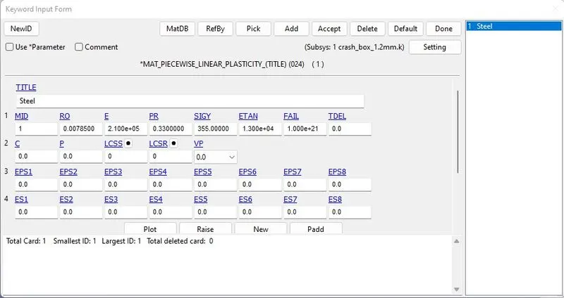
Fig 5: The material property is assigned with appropriate material law for the crash box.

• Hourglass phenomena are expected in the shell elements; to avoid this hourglass effect, the hourglass keyword with Flanagan-Belytschko viscous form is added to take care of it.

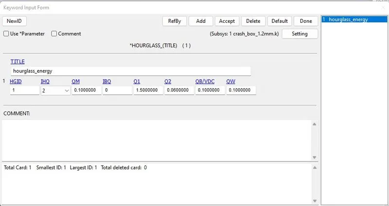
Fig 6: hourglass effect is controlled with this keyword.

• The material, hourglass form, and element formulation should be assigned to the crash box part we have created earlier.

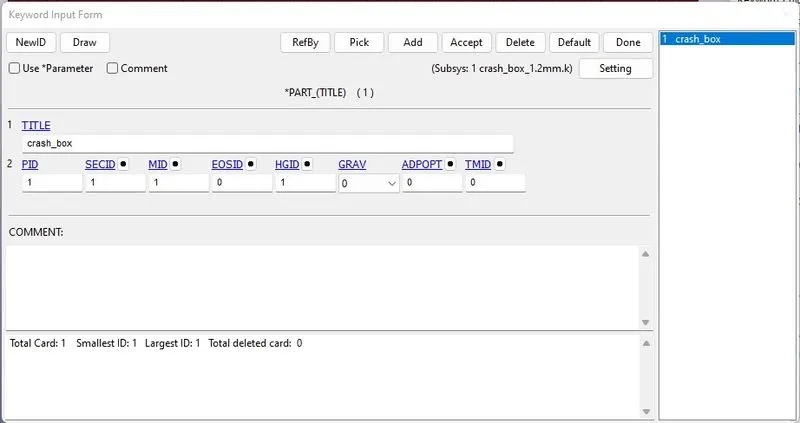
Fig 7: Material and section along with hourglass control are assigned to the crash box.

• To provide initial velocity to the crash box, the velocity keyword from the initial deck is chosen. Entering the node-set id and the velocity value in the x-direction with a value of -13.88 defines it ultimately.

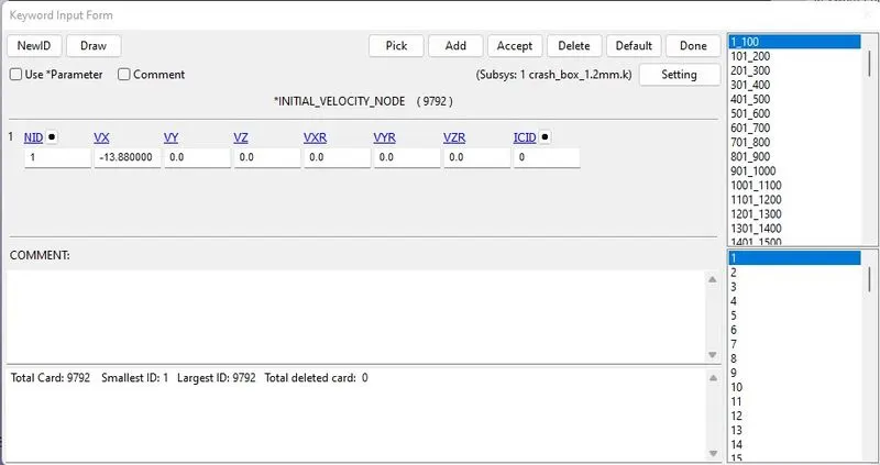
Fig 8: Velocity is defined for the crash box.

• Navigate to Model>Create entity options from the right hand menu ribbon. In the Rigidwall option from the Rigidwall drop-down, we create a rigid wall with a planar cross-section with the 1n+NL option checked.

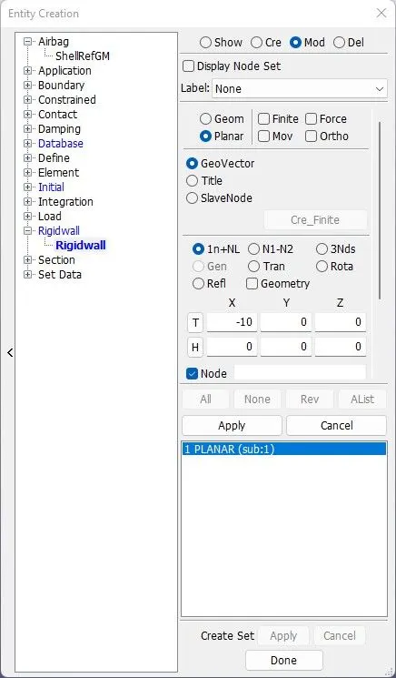
Fig 9: A rigid wall is created with these inputs shown.

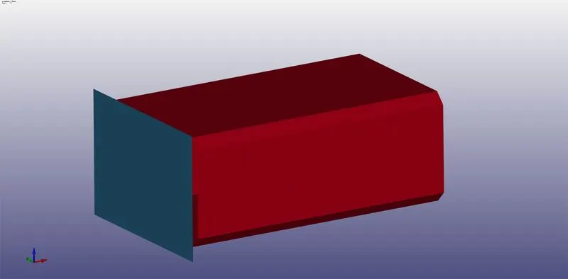
Fig 10: Rigid wall boundary created in front of the crash box

• AUTOMATIC_SINGLE_SURFACE contact card is defined with the static and dynamic friction coefficient values of 0.008.

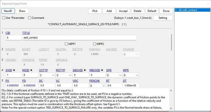
Fig 11: Contact is established for the crash box if it comes in contact with itself during the crash.

• The ASCII_option keyword from the DATABASE deck is used for the output requests, and GLSTAT, MATSUM, NODOUT, RCFORC, RWFORC, SECFORC, and SLEOUT options are checked.

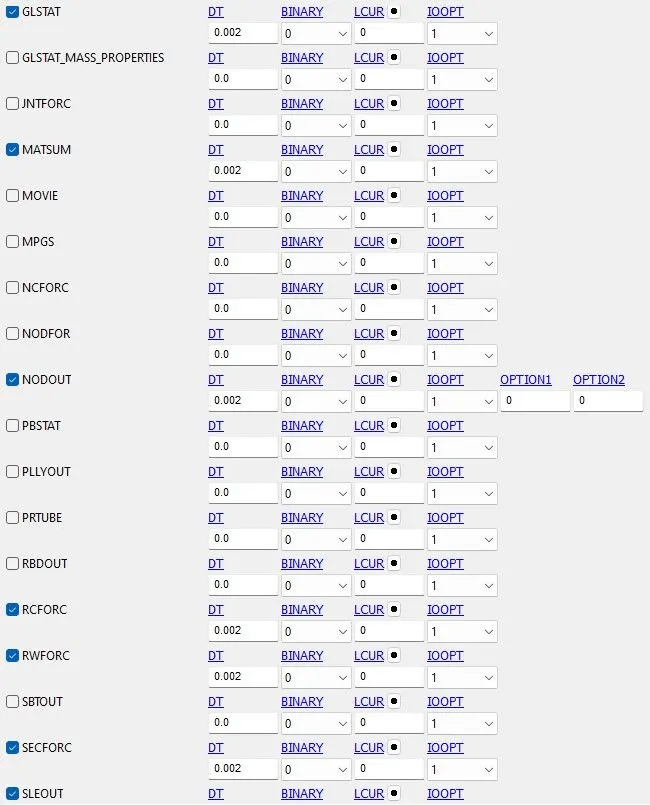
Fig 12: Output requests are defined.

• The BINARY_D3PLOT keyword from the DATABASE deck is used for the plots, and a DT of 0.002 is entered.

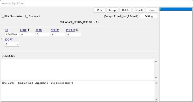
Fig 13: Plots at time intervals are defined.

• DATABASE_EXTENT_BINARY card with STRFLG =1 is used to compute the elastic strain in the model.

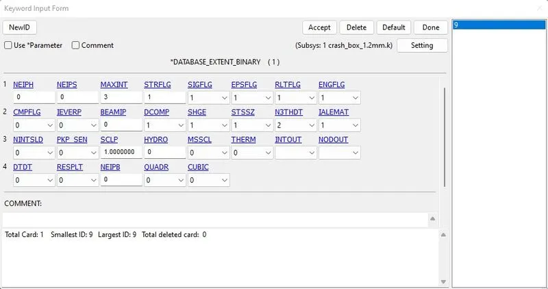
Fig 14: Elastic strain computation is enabled.

• Navigate to Model>Create entity options from the right hand menu ribbon. In the Cross section option from the Database drop-down, we create a plane cross-section with the 1n+NL option checked.

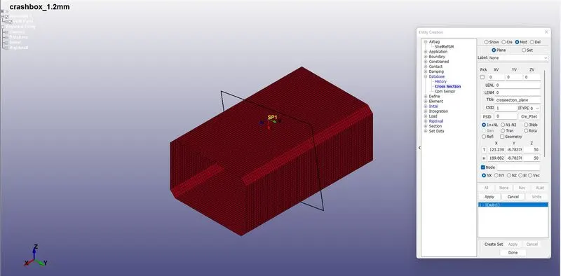
Fig 15: Cross-section is created in the middle of the crash box.

• DATABASE_CROSS_SECTION_PLANE card is used to compute forces at that particular section.

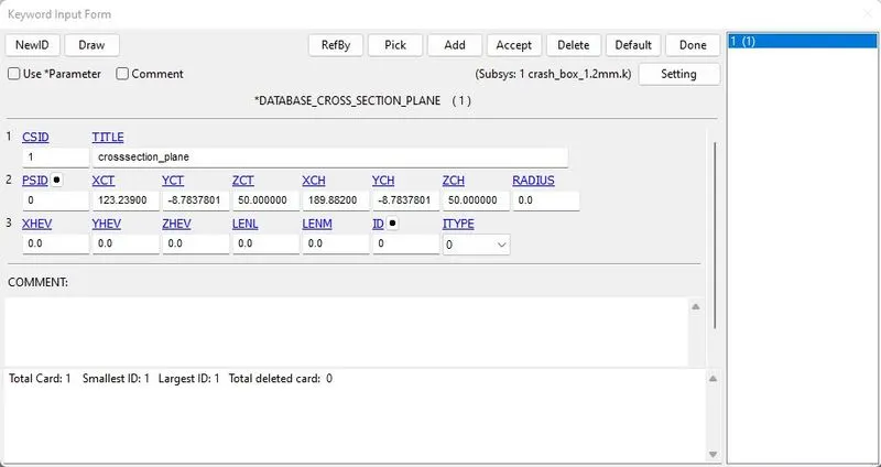
Fig 16: Cross-section card is defined.

• HISTORY_NODE keyword is used from the DATABASE deck to compute the acceleration of node 5094.

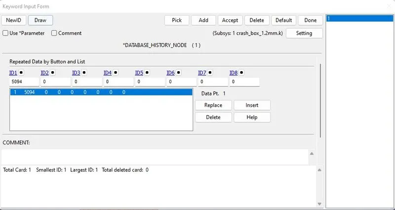
Fig 17: Node is created to compute the acceleration.

• Finally, the TERMINATION keyword from the CONTROL deck is used to define the end time of the simulation.

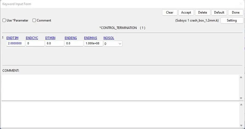
Fig 18: End time for the simulation is defined.

• With all these keywords included, the deck is fully defined and is now ready to solve.

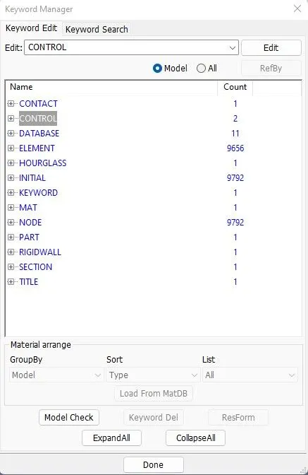
Fig 19: Fully defined deck for the drop test.

• Open the Start LS-Dyna analysis, browse the keyword file, and hit run to run this keyword file.

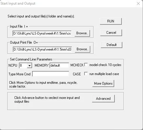
Fig 20: LS-Dyna analysis browser.

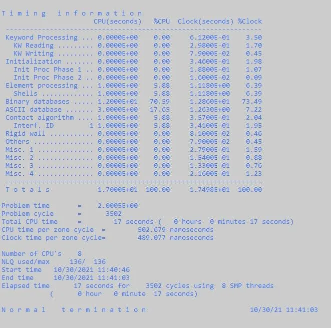
Fig 21: Successful completion of solving.

• Open new LS-PRE POST from the launch manager and open the LS-DYNA Binary plot (choose the D3PLOT file created) from the file menu.
• The model will be loaded the same as before, but we can access only the post-processing options from the right ribbon menu.

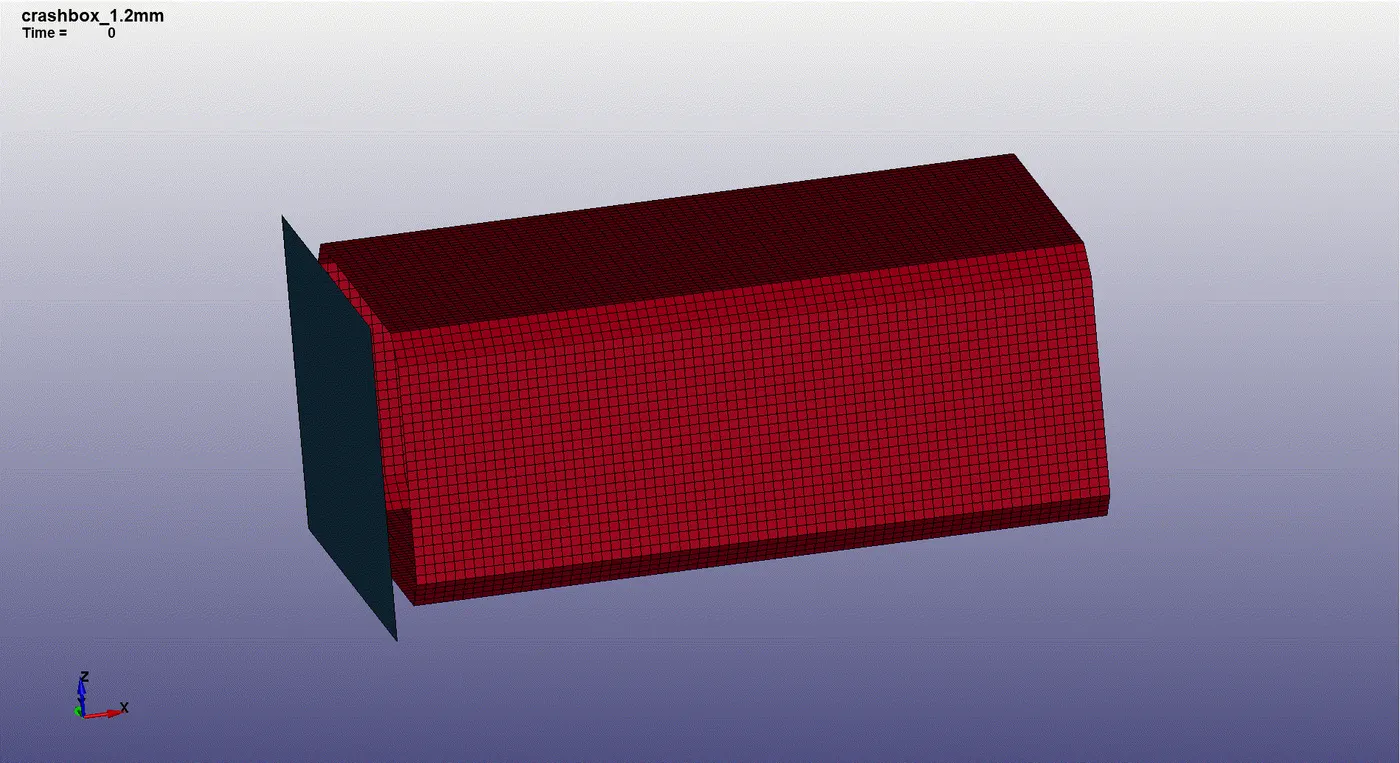
• The above animation represents the crash box with a thickness of 1.2mm, hitting on the wall and rebounding.

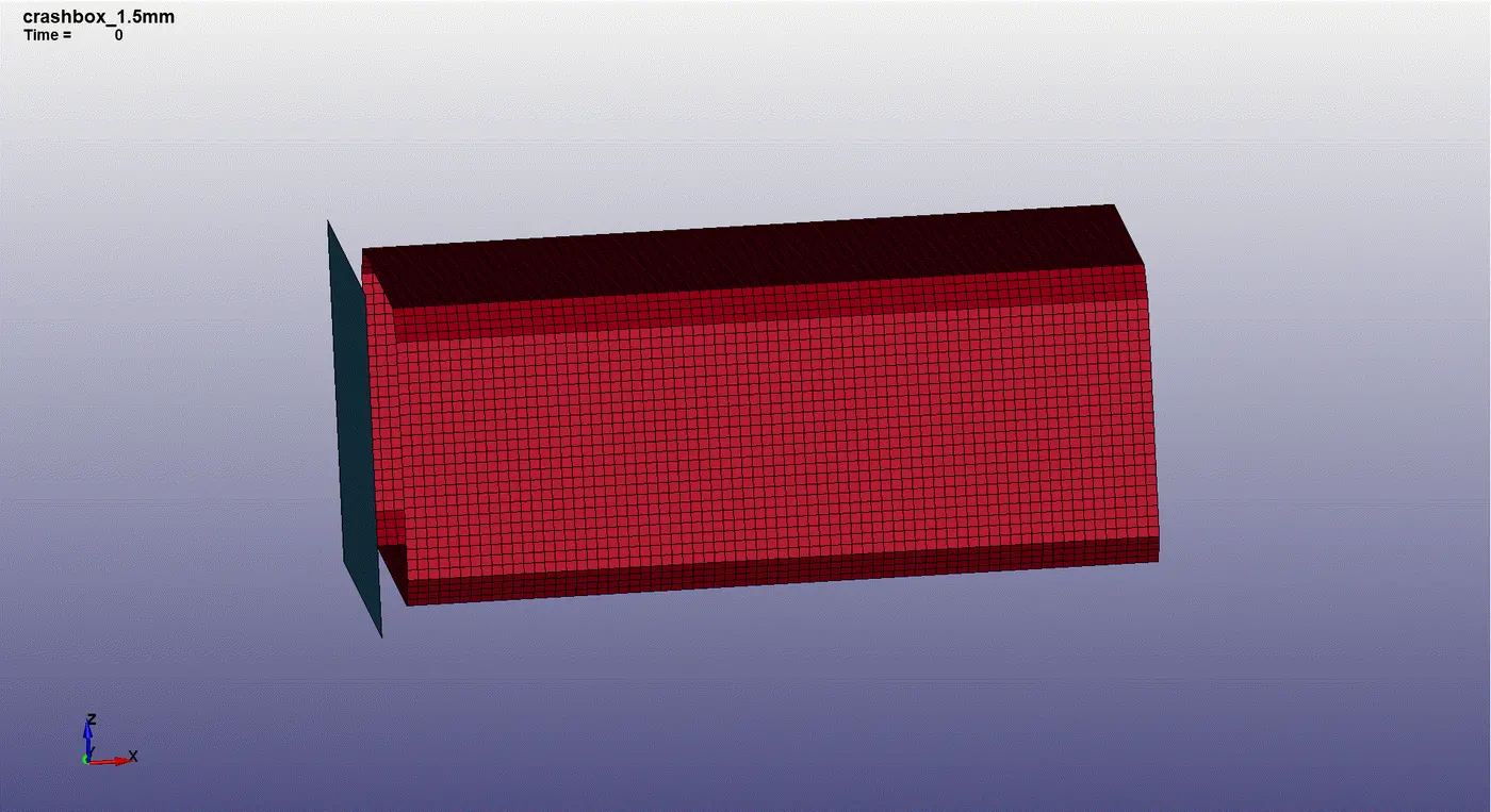
• The above animation represents the crash box with a thickness of 1.5mm hitting on the wall and rebounding.
• Within the Fringe Component, multiple quantities are listed to visualize the contours.

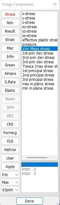
Fig 22: Fringe component menu.

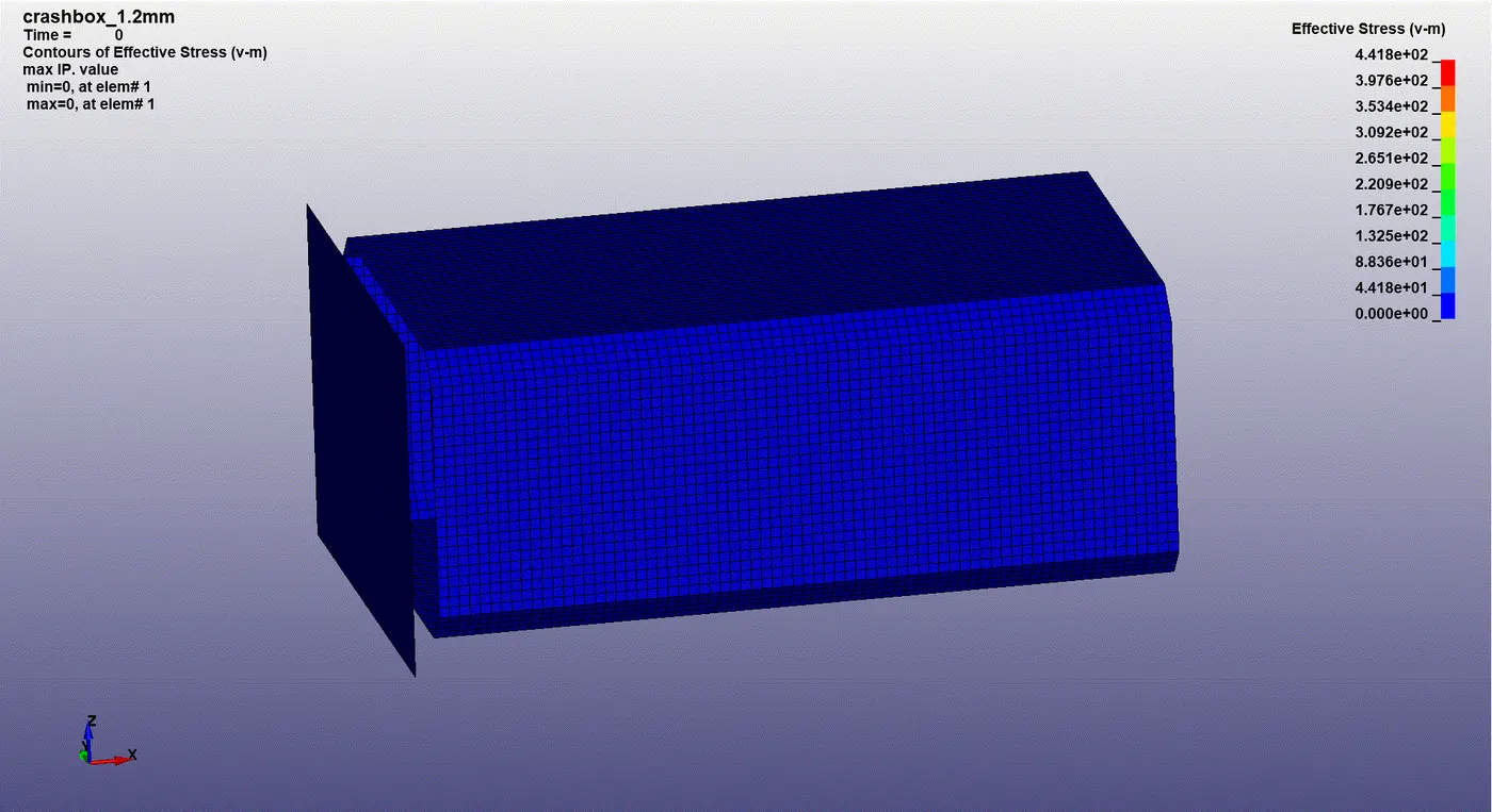
• The above animation shows the von-mises stresses produced in the crash box with a thickness of 1.2mm due to the crash.

• The above animation shows the von-mises stresses produced in the crash box with a thickness of 1.5mm due to the crash.

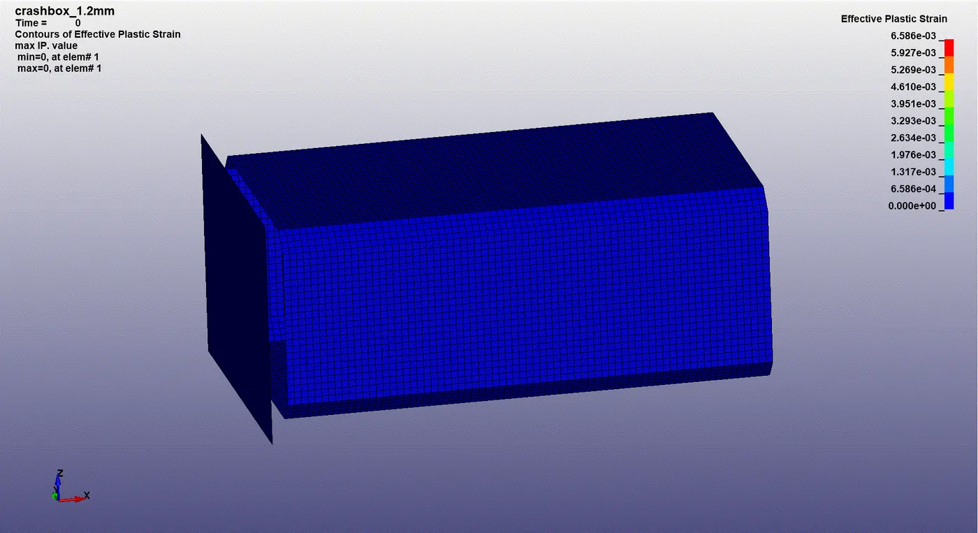
• The above animation shows the effective plastic strain produced in the crash box with a thickness of 1.2mm due to the crash.

• The above animation shows the effective plastic strain produced in the crash box with a thickness of 1.5mm due to the crash.
• Navigate to the ASCII option from the right ribbon to plot the different variables, and a separate menu pops showing the output requests.

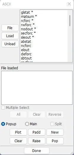
Fig 23: ASCII options for plotting the graphs.

• Each output request has different data quantities available within them to plot. Whatever file is required, it is loaded first, and the required quantities are chosen for plotting.

Energy Plots:

The kinetic, internal, total, hourglass, and sliding energy were plotted for 1.2 mm and 1.5 mm thick crash boxes. The graph depicts the energy balance of a dynamic test on a crash box; as the kinetic energy decreases, the internal energy increases. The other important things to consider are that the total energy must remain constant, and the sliding interface must remain low.

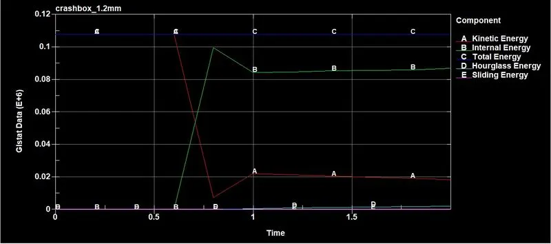
• The above graph represents the kinetic, internal, total, hourglass, and sliding energy available in the GLSTAT for the thickness of the 1.2mm crash box.

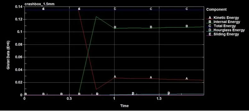
• The above graph represents the kinetic, internal, total, hourglass, and sliding energy available in the GLSTAT for the thickness of the 1.5mm crash box.
• The Energies are more eminent for the 1.5 mm thick crash box. The total energy for the 1.2 mm thick and 1.5 mm thick crash box was recorded as 0.114E+6 N-mm and 0.134E+6 N-mm, respectively.
• At 0 ms, the whole of the total energy is Kinetic energy. But as the simulation progresses and the impact between the Crash box and the Rigid wall takes place, at approx 0.6 ms, the Kinetic energy starts getting converted into Internal energy.
• The Internal energy reaches its peak, and the kinetic energy comes at its lowest value at about 0.79 ms when the crash box is on the verge of getting rebounded from the rigid wall.
• The crash box then moves with a constant rebound velocity reflected in the energy plot as internal energy gets converted to kinetic energy and remains constant throughout the simulation.

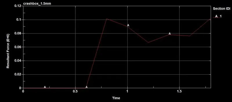
Sectional Forces:

• Sectional force in a 1.2mm thick crash box.

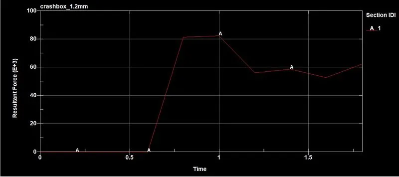
• Sectional force in a 1.5mm thick crash box.

Acceleration in node 5094:

• Acceleration produced in node 5094 for the 1.2mm thick crash box.

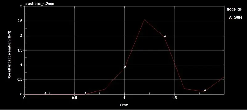
• For the 1.2mm thickness crash box, the resultant acceleration is developed during the collision with a rigid wall and increases to a maximum of 2.56x E+3 mm/ms at time 1.24 ms and decreases while the crash box is rebounded.
• Acceleration produced in node 5094 for the 1.5mm thick crash box.

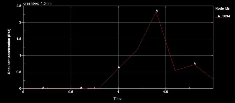
• For the 1.5mm thickness crash box, the resultant acceleration is developed during the collision with a rigid wall. It increases to a maximum of 2.4E3 mm/ms at a time of 1.4 ms and decreases while the crash box is rebounded.

Maximum directional stress and strain along the length of the crash box:

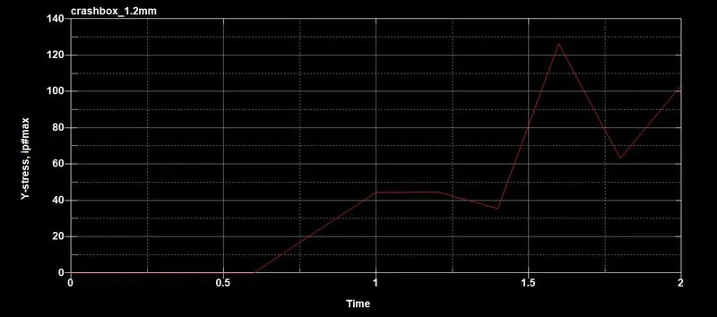
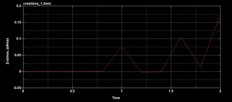
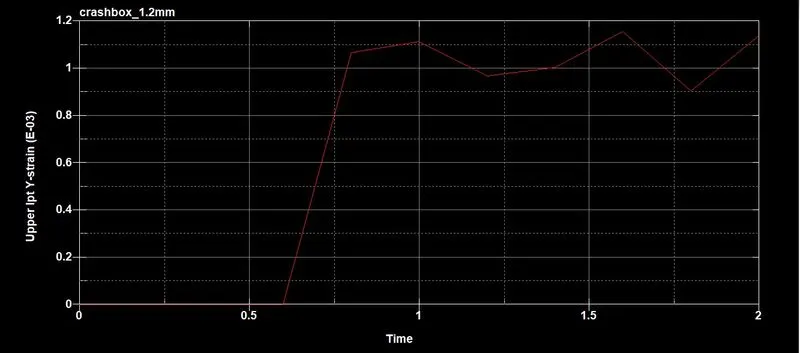
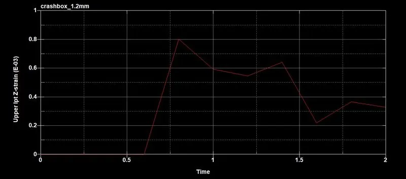
• The directional stress and stain in the x, y, and z-stress are plotted for the crash box with 1.2 mm thickness.
• The maximum stress in x, y, and z directions with 1.2mm thickness:

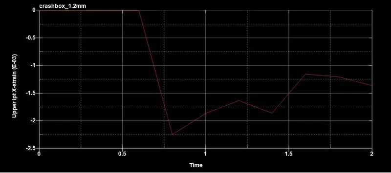
• The maximum strain in x, y, and z directions with 1.2mm thickness:

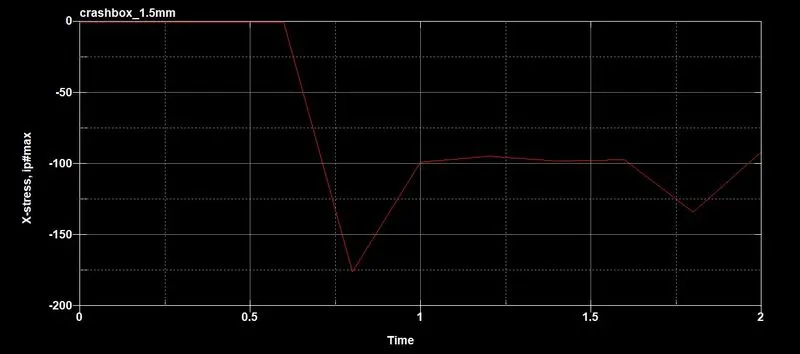
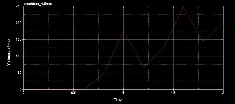
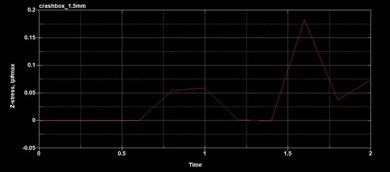
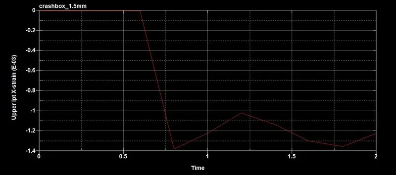
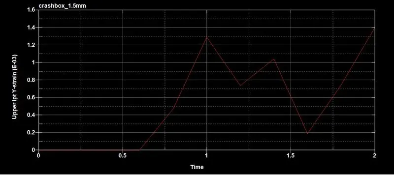
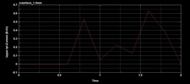
• The directional stress and stain in the x, y, and z-stress are plotted for the crash box with 1.5 mm thickness.
• The maximum stress in x, y, and z directions with 1.5mm thickness:

• The maximum strain in x, y, and z directions with 1.5mm thickness:

Conclusions:

• The solver deck was set up for the crash simulation, and the needed results were requested using the appropriate *DATABASE keyword cards.
• The results are compared for both 1.2 mm and 1.5 mm thick crash boxes.
• The results of the 1.5 mm crash box showed higher energy absorbing capacity and more minor deformation compared to 1.2 mm thickness crash box.