Week 4 - CHT Analysis on Exhaust port
- CHT Analysis on Exhaust port]
CHT, conjugate heat transfer refers to the combination of conduction, convection and radiative heat transfer in the surrounding fluids. whenever the solid and fluid interface appears and there is an exchange of thermal energy between them, the CHT analysis can be performed.
Conjugate heat transfer investigation helps in determining the surface temperatures and heat exchanging abilities of the devices. Through this analysis, engineers can optimize the thermal parameters for their design.
Some are examples of where CHT analysis can be performed
- Internal combustion engines - The internal combustion engine industry is moving towards the simulation of the entire system rather than independent components. the accuracy of the predicted combustion in the cylinder is depended on the temperature boundary conditions in the cylinder. By considering the heat transfer coefficient in the metal components the cylinder wall no longer has a user-specified temperature but has temperature predicted as part of the complete system simulation. this makes overall simulation results more predictive by reducing the dependence on assumed boundary conditions.
- Electric Vehicle - As we know the revolution in electric vehicles has been started to make it more sustainable we should consider, the effective cooling strategies of various components of the systems. Electric motors have high power densities and thus generate a significant amount of heat if a motor is not properly cooled, high temperature in the motor can cause the demagnetization of permanent magnets and lead to the breakdown of winding insulation.
- Pumps and compressor - Resolving the spatially varying surface temperature distributions in pumps and compressors improves the accuracy of the simulation and provides useful temperature data. For example, in a twin-screw compressor, thermal expansion affects the clearance between the rotors. If that effect is not captured, the simulation will incorrectly predict leakage flows and lower the accuracy of your results.
- Boiler and Heat process equipment- Boilers and process equipment are employed under high temperature and high-pressure conditions breakdown of a boiler can lead to huge losses, energy as well as economical loss. The water inside a boiler gets heated with the flames coming from the burner resulting in the water boiling and creating high temperature and pressure. By CHT we can predetermine the heat transfer between the fluid and the boundary wall. Analysis can avoid the flow eddies and give results where the system getting overheated hence breakdown can be avoided.
SETUP
1. Geometry
- Load the CAD model in SpaceClaim & change units from mm to m.
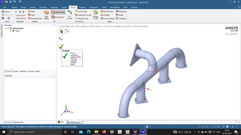
- As the geometry is complex there might be extra unwanted edges that will further give problems during mesh, so to resolve it have to select the option extra edges.
- SpaceClaim provides manual selection as well as auto-selection of extra edges by clicking the green check all the extra edges will be deleted.
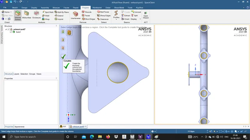
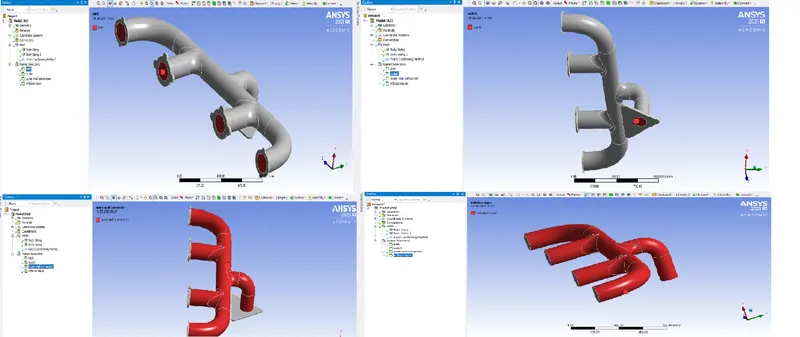
- Flow from the exhaust pipe has to derive from 4 inlets towards 1 outlet therefore we have to create a volume of the flow.
- To creat the flow Clame->Prepare->Volume extraction->Selecting edges of inlet and outlet ports->Click green tick.
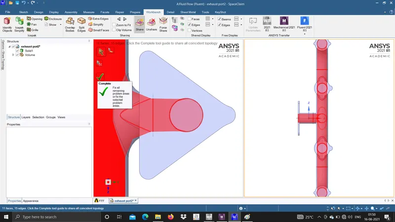
- As it is a CHT analysis we have to confirm the flow relates to the solid surface as well so we have to share topology where the mesh gets connected and results in a fine mesh.
- To share select the Share from the workbench and SpaceClaim autogenerates the two share surface volume and edges as shown in the above figure.
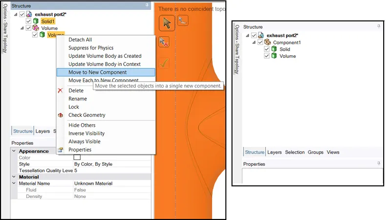
- Now, as shown in the above figure select the objects and replace the previous objects in the new component and delete the empty component and name the objects as solid and fluid volume.
- Update the SpaceClaim and close SpaceClaim
2. MESHING
Calculating Y+
- Calculating Re
we know that,
`U=5`
`D=0.17`
`mu=0.000017894`
`rho = 1.225`
`Re = (rho*U*D)/mu`
`therefore Re= 58189.89`
- calculating cf
`Cf=0.026/(Re^(1/7))`
`therefore Cf=0.005423`
- calculating shear stress near-wall
`tau_w=(Cf*rho*u^2)/2`
`therefore tau_w=0.0830`
- Friction velocity
`U_f=(tau_w/(rho))^0.5`
`therefore U_f= 0.2603`
- calculating first layer thickness For Y+ 50
`Delta Y=(y+ *0.000017894)/(1.225*0.2603)`
`therefore DeltaY=0.002803`
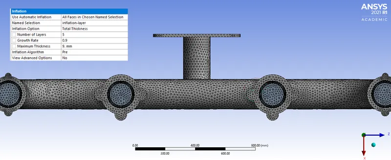
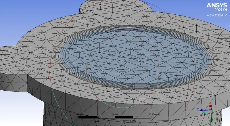
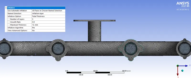
- Thickness for 5 layers with Gr 0.9.
- `T_l=DeltaY*Gr^(n-1)`
| Sr. | n | thickness in mm |
| T1 | 5 | 1.84 |
| T2 | 4 | 2.04 |
| T3 | 3 | 2.27 |
| T4 | 2 | 2.52 |
| T5 | 1 | 2.80 |
| TOTAL THICKNESS | 8.67 ie. 9mm |
- Total inflation layer thickness for various y+ values
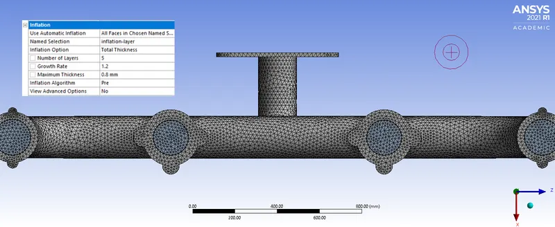
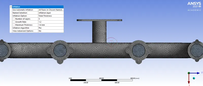
Case For k-epsilon model Case A- Growth rate 0.9 1A Y+ 50 9mm 2A Y+75 12mm For k-omega model For Case B - Growth rate 1.2 1B Y+2 0.8mm 2B Y+4 1.6mm
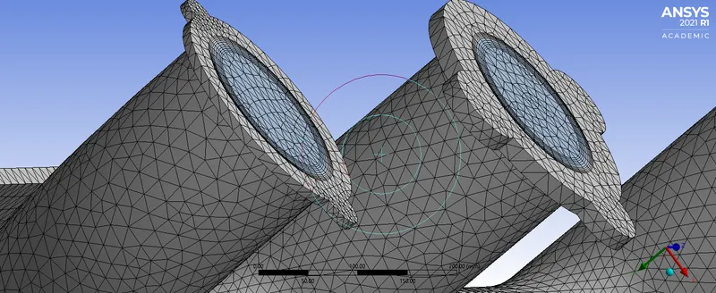
- Open mesh and name the selections for Inlet, outlet, Outerwall-convection & inflation layer respectively as shown in below figure.
CASE A
- Inflation layer
|
Case 1A |
|
 |
 |
| Case 2A | |
 |
 |
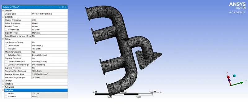
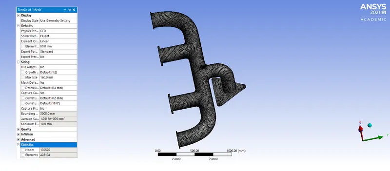
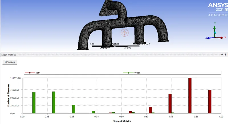
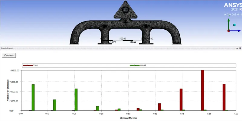
- Number of element
|
 |
|
||||||||
|
 |
|
- Element size
| Case 1A |
 |
| Case 2A |
 |
CASE B
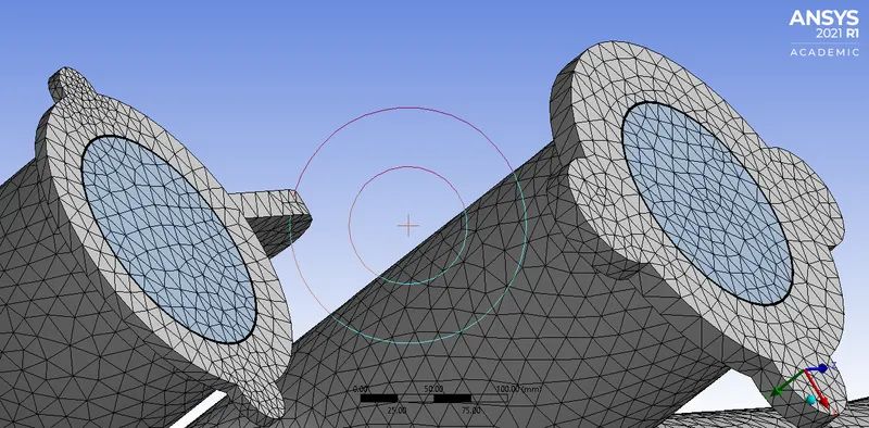
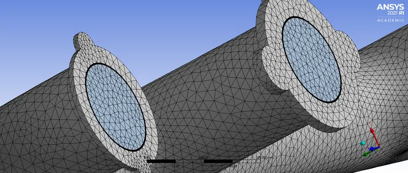
- Inflation layer
|
Case 1B |
|
 |
 |
| Case 2B | |
 |
 |
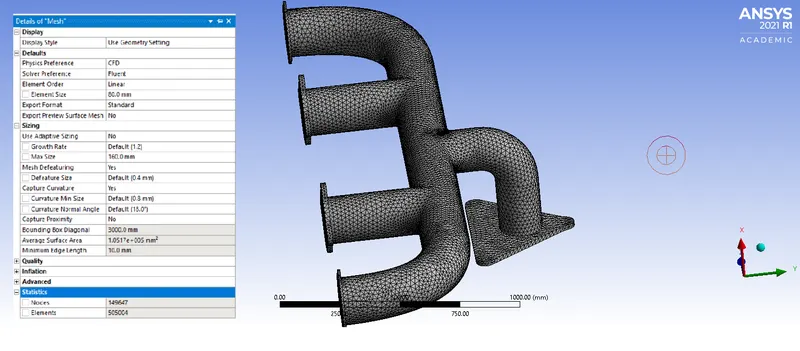
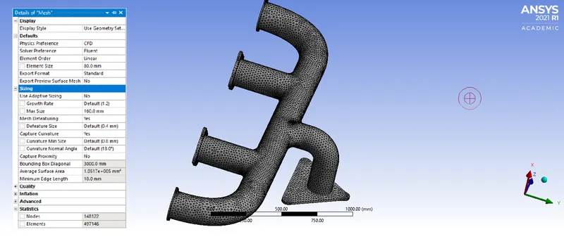
- Number of element
|
 |
|
||||||||
|
 |
|
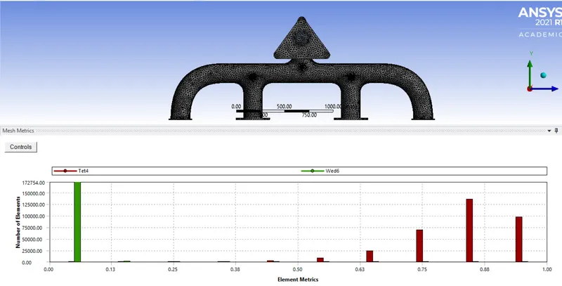
- Element size
| Case 1B |
 |
| Case 2B |
| |
- SETUP
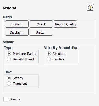
Using pressure-based solver we have to perform all cases.
General setting; After mesh -> update mesh and open fluent with double precision.
check the mesh and proceed for further set up as follows.
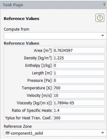
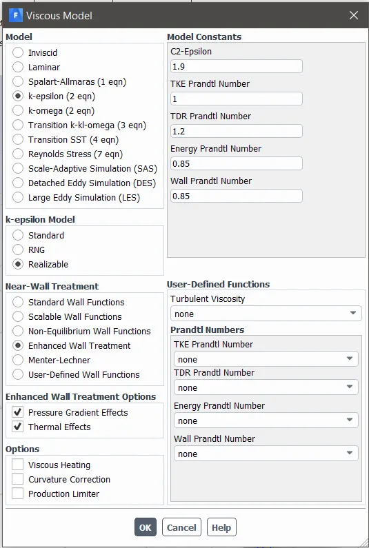
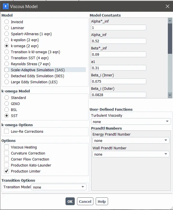
PHYSICS
|
 |
|
 |
|
 & &  |
&
|
|
|
|
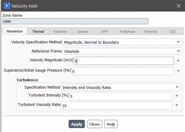 &
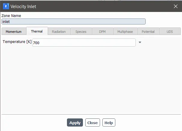
&
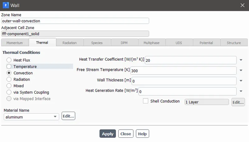
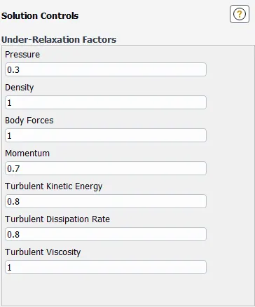
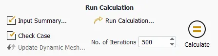
SOLUTION
|
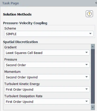 |
|
 |
|
 |
|
 |
RESULTS
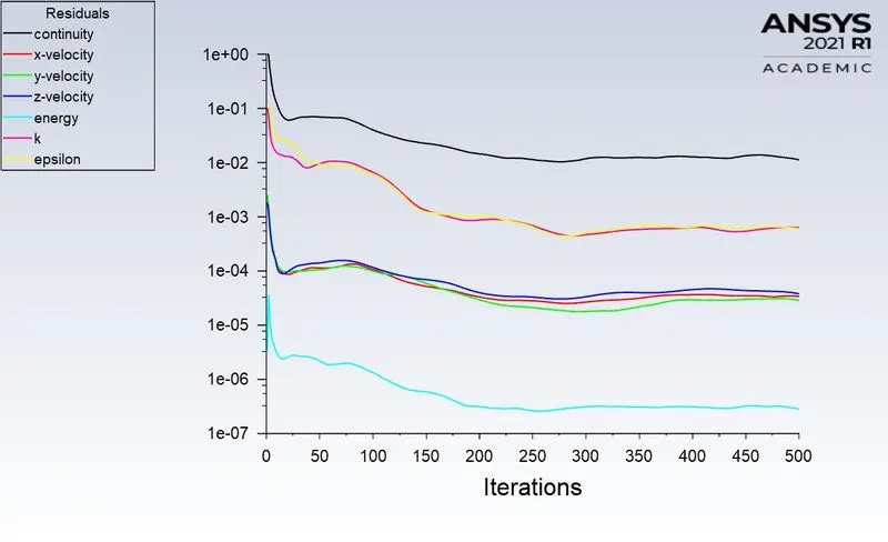
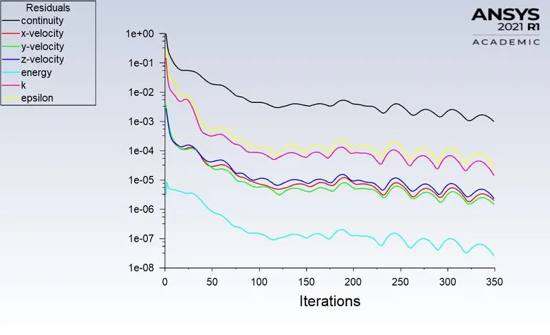
- Scalar residuals
| Case A K-epsilon Realizable | |||
|
Case 1A Y+50 |
 |
Case 2A Y+75 |
 |
| Case B K-omega SST | |||
|
Case 1B Y+2 |
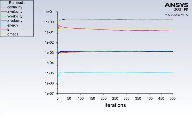 |
Case 2B Y+4 |
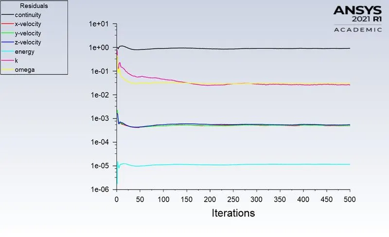 |
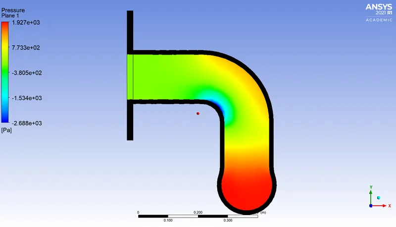
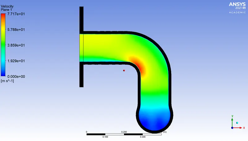
- Case A
| Case 1A | |
|
Pressure
|
Velocity
|
|
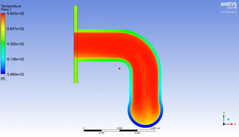
Temperature
|
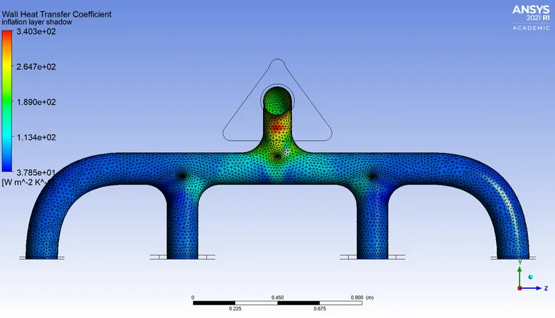
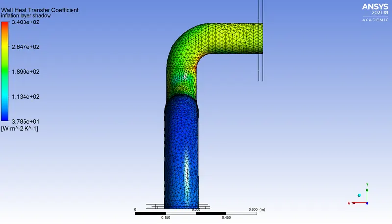
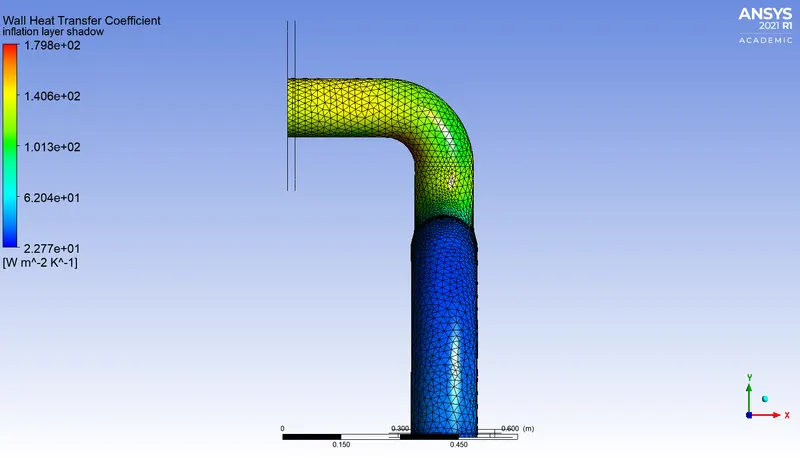
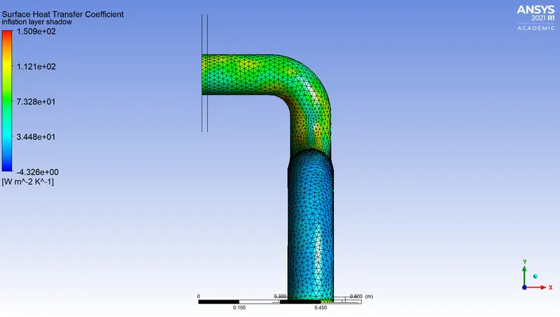
Wall heat transfer coefficient
 |
 |
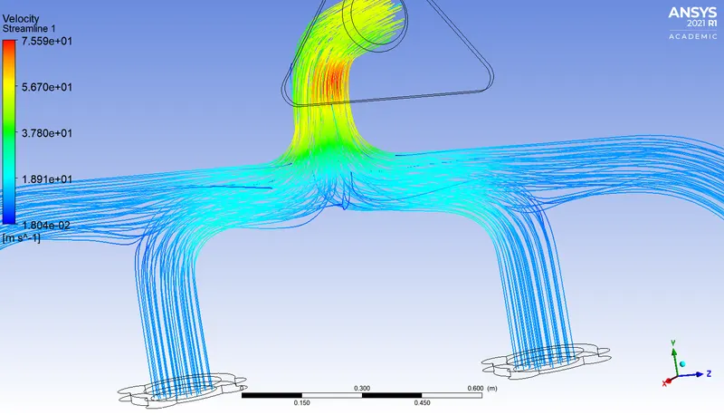
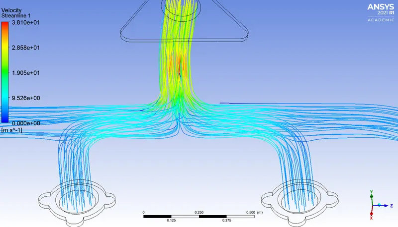
| Streamline |
 |
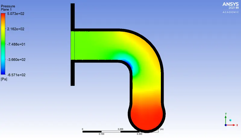
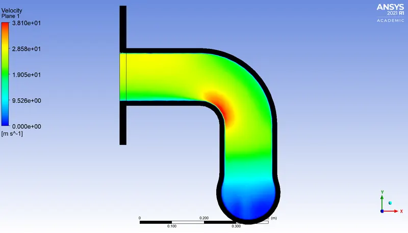
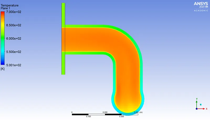
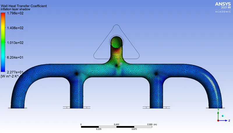
| Case 2A | |
|
Pressure
|
Velocity
|
|
Temperature
|
Wall heat transfer coefficient
 |
 |
| Streamline |
 |
Case B
| Case 1B | |
|
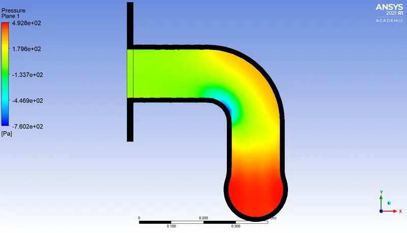
Pressure
|
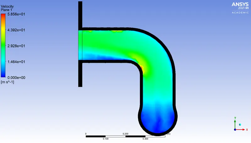
Velocity
|
|
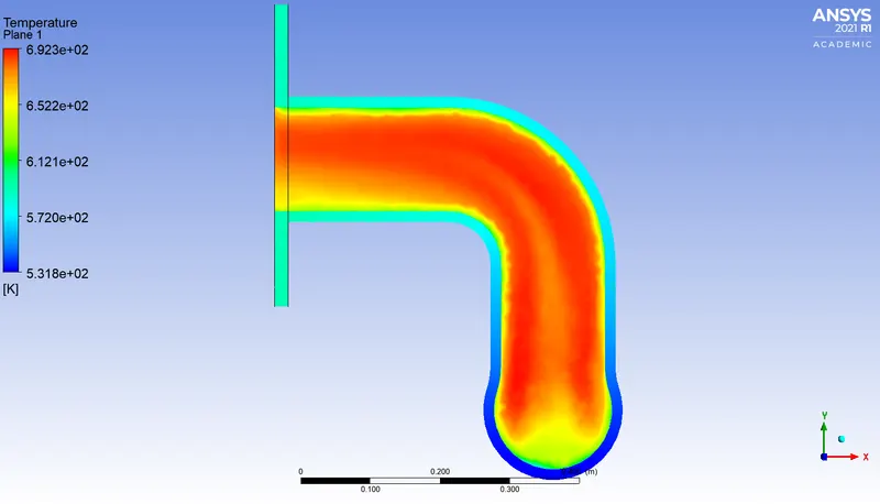
Temperature
|
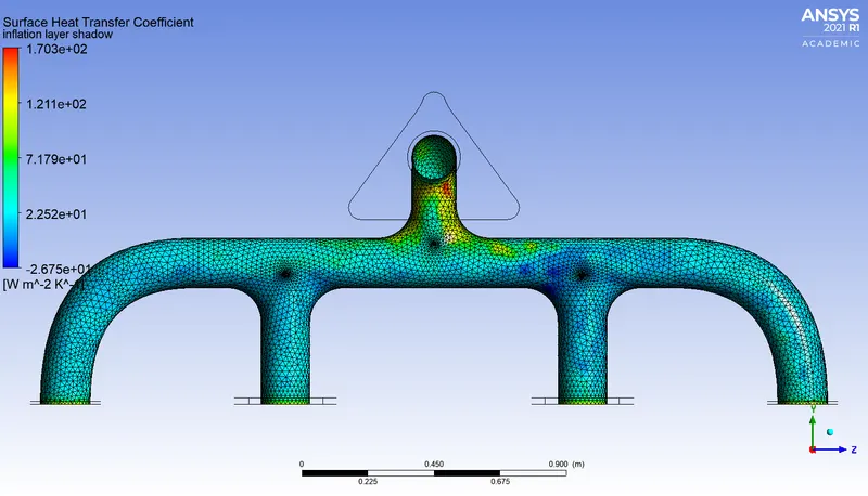
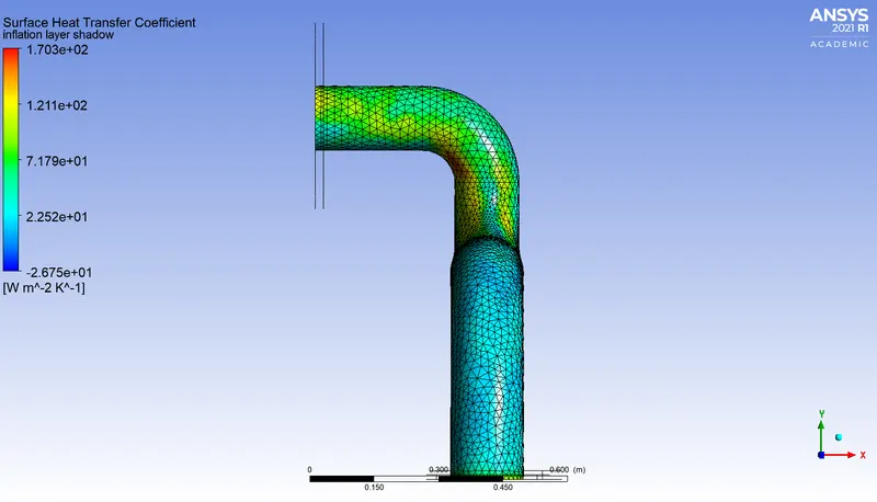
Wall heat transfer coefficient
 |
 |
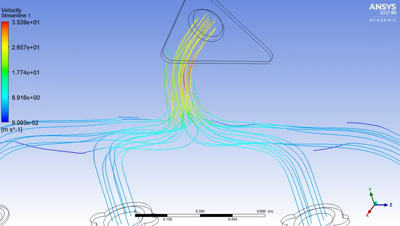
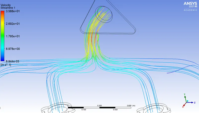
| Streamline |
 |
| Case 2B | |
|
Pressure
|
Velocity
|
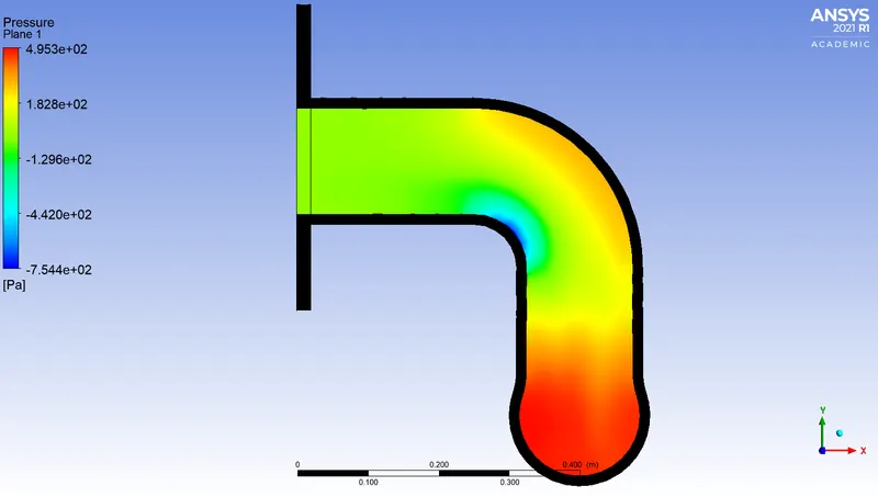
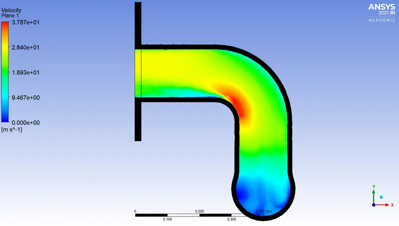
|
Temperature
|
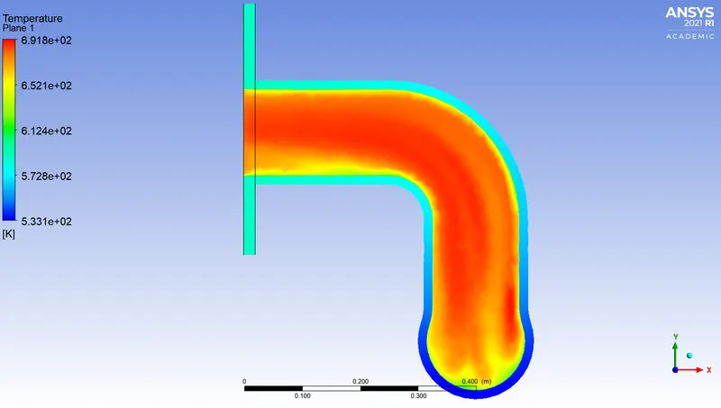
Wall heat transfer coefficient
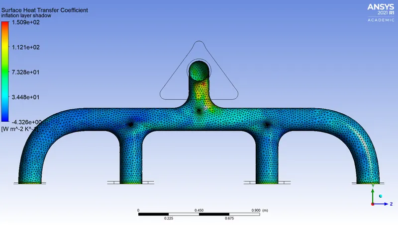 |
 |
| Streamline |
 |
Conclusion
- Mesh/ grid dependency test is very important to get confidence over results.
- You can validate your experimental work and the numerical results with another work to understand the over all phenomena.
- For the turbulent models, we have to take care of the assumptions and the boundary conditions we put in the program. The mesh is a very important parameter to get good results, that's why we have to refine it in the important place of our geometry
- Some factors that should be considered which are the most significant is the turbulent boundary layer. If we are using any kind of low Reynolds turbulence model considering enhanced wall treatment (as our K-w SST model), so we need to make sure that we stay in the laminar sub-layer region where velocity profiles are assumed to be laminar and viscous stress dominates the wall shear.
- Understanding from this simulation, the main motivation behind the development of omega-based models has been to address some shortcomings of the k-epsilon model in dealing with near-wall phenomena. As a result, it seems intuitive, those omega-based models should require a high-resolution mesh in the vicinity of the wall (i.e. y+ ~ 1) to fully resolve the boundary layer all the way down to the wall; the objective for which omega-based models were originally developed.
- In the fluent software, the value of the convection heat transfer coefficient extremely depends on the reference temperature. you should use the proper bulk temperature as the reference temperature.