Week 4 - CHT Analysis on Exhaust port

Abstract:

The following study is a conjugate heat transfer analysis of an exhaust manifold and in turn calculating or predicting the wall heat transfer coefficient. The temperature, velocity distribution plots are shown . Two cases are analysedmwith different mesh sizes.

key words : CFD, exhaust manifold , CHT , infkation layers, y+ , CFD post, Wall heat transfer coefficient

Introduction:

Conjugate heat transfer corresponds with the combination of heat transfer in solids and heat transfer in fluids.Conjugate heat transfer is observed in many situations. For example, heat sinks are optimized to combine heat transfer by conduction in the heat sink with the convection in the surrounding fluid. The Conjugate Heat Transfer (CHT) analysis type allows for the simulation of heat transfer between solid and fluid domains by exchanging thermal energy at the interfaces between them. Typical applications of this analysis type exist as, but are not limited to, the simulation of heat exchangers, cooling of electronic equipment, and general-purpose cooling and heating systems.

Flow-chart of the analysis:

• Geometry import
• Geometry preparation
• Meshing
• Mesh refinement
• Physics set up ( boundary conditions, turbulence modelling, solver settings)
• Post-processing in CFD-post

Baseline simulation:

• Geometry:

A cad model of exhaust manifold is imported into space claim.

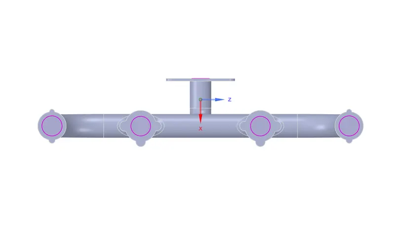
The three views of the exhaust mainifold are :

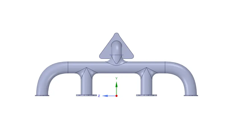
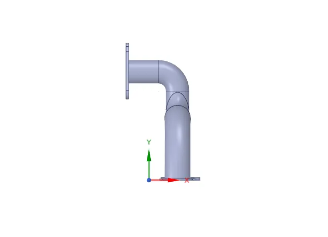
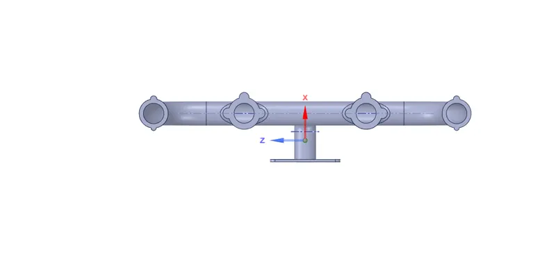
The next step is to extract the fluid volume. This is done by using the prepare option, edge selection is opted and the fluid volumes are extracted.

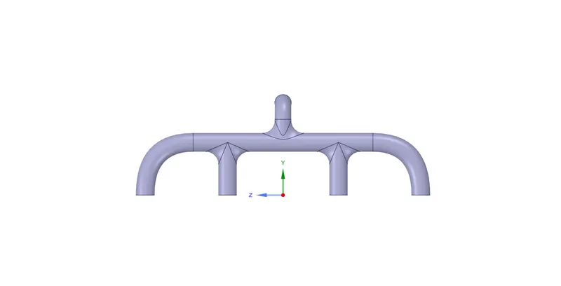
There are interfaces or surfaces where the fluid volume and the solid shares . This should be made to share or enabled to share using the share prep option in the workbench.

The components solid and fluid volume are selected and moved to a new component and named final geometry. Shared topology is enabled.

• Meshing:

Since it is a base line simulation. The default meshing that ansys mesher does is checked. Named selections are provided to all the parts so that boundary conditions can be applied when physics is set up. There are three named selections - inlets, where from the exhaust hot gases enters the exhaust manifold, outlet, from where the exhaust gases exit, convection walls .

1) Baseline simuation:

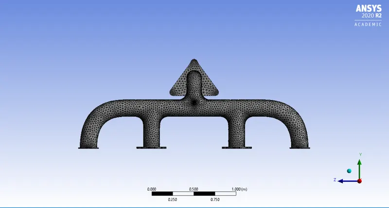
• Meshing parameters:

element size : 0.15 meters

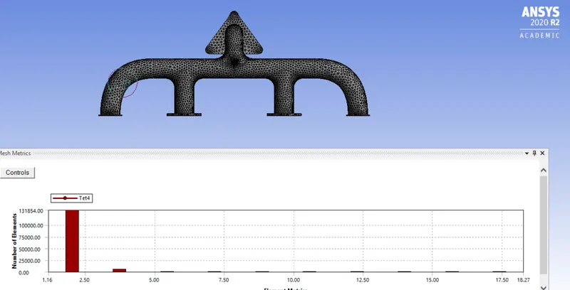
aspect ratio :

minimum	1.1609
maximum	18.27
average	1.9015
standard deviation	0.49844

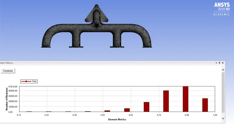
skewness:

minimum	6.674e-005
maximum	0.89547
average	0.25187
standard deviation	0.12817

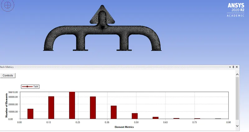
Orthogonal quality:

minimum	0.10453
maximum	0.99133
average	0.74673
standard deviation	0.12622

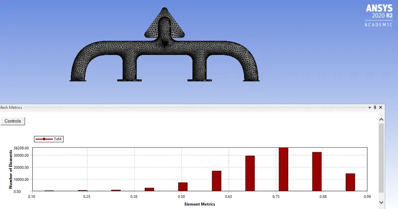
Statistics:

elements	137570
nodes	27438
element size	0.15 meters

• Solution:

1)Set-up:

The mesh is updated and fluent set u is openned. Double precision is turned on and 4 processors are assigned.

• Physics:

while loading the meshing data from the ansys mesher , fluent may flag some errors that might happen due to creation of duplicate cell zones and can be rectified from the recorded mesh data file.

The materials assigned is checked, For the Fluid it is air and the solid part is constituted of Almunium.

properties of air and almunium:

air:

density	1.225
c_p	1006.43
thermal conductivity	0.0242
viscosity	1.789e-005

Almunium:

density	2719
c_p	871
thermal conductivity	202.4

All units are in SI system.

Operating conditions:

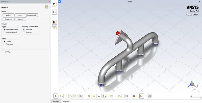
Pressure based solver is used. Velocity formulation is absolute and perpendicular to the boundary . Steady state analysis is performed. Since the study is dealt wit in horizontal condition, no gravity is turnd on.

Solution methods:

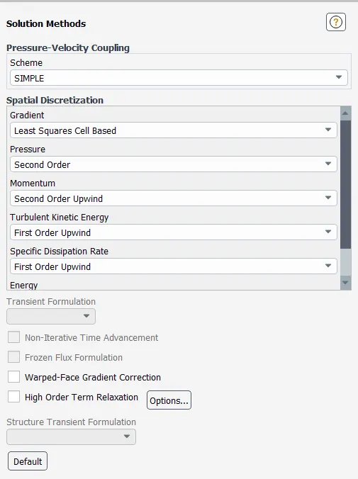
The pressure velocity coupling is selected as SIMPLE scheme.

Boundary conditions:

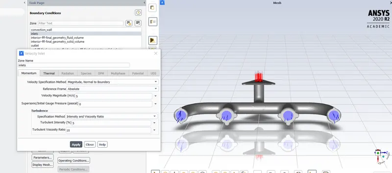
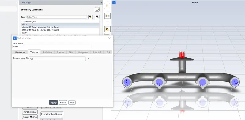
• inlets:

For the inlets, the velocity of fluid inflow is taken as 5m/s (hot fluid). The temperature of the fluid taken as 700K.

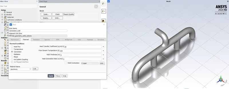
• convection wall:

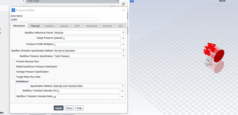
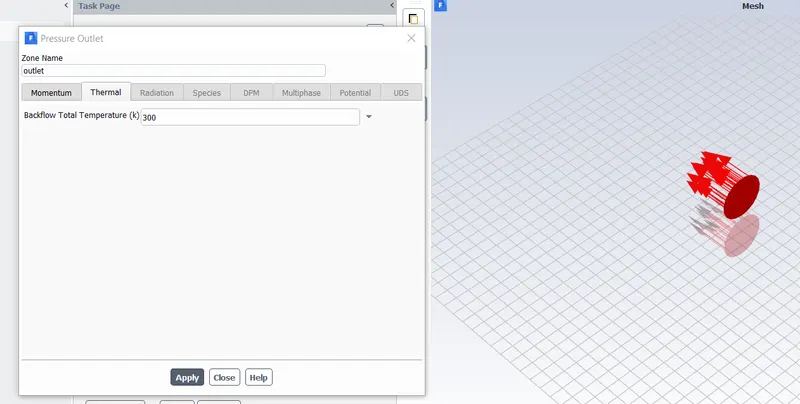
• outlet:

This has basically a pressure bundary conditions

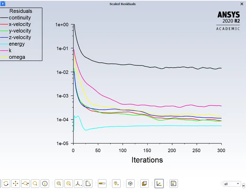
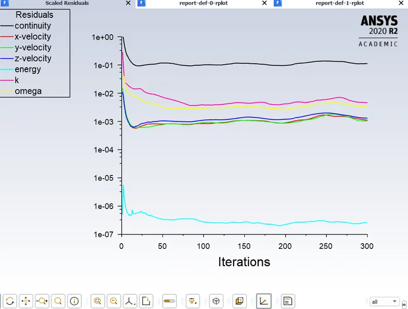
Hybrid initialisation is done. The solution is run for 300 iterations.

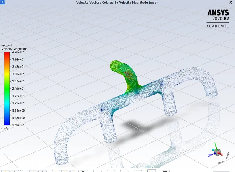
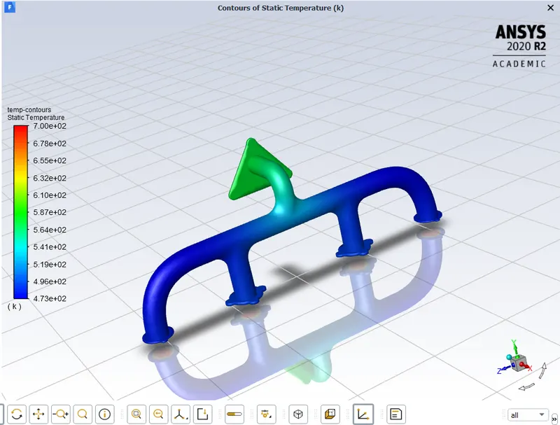
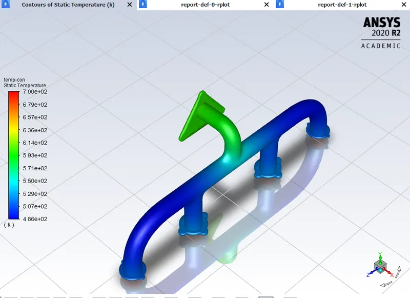
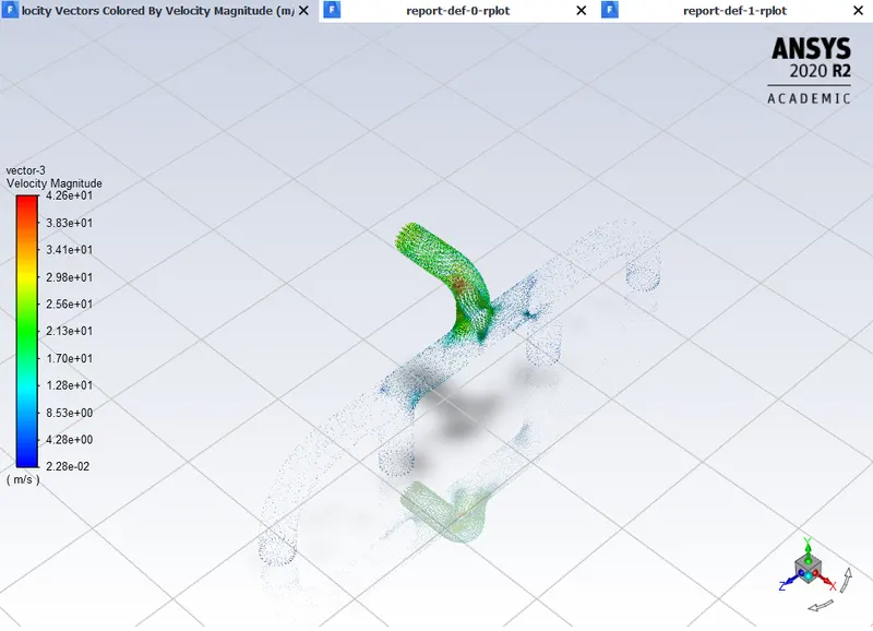
A velocity vector plot, temperature contour is created.

• Post-processing:

CFD-post is a post processing tool used to visualize the results obtained from the simulation.

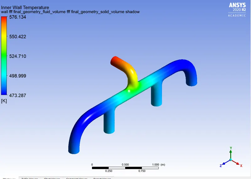
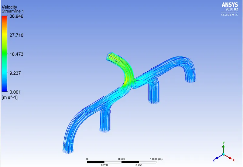
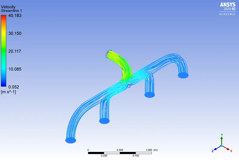
From the streamlines plot of the velocity it is visualized that the the velocity is more at the throat section of the outlet. It can be attributed to the fact the the conservation of mass is maintained. The collective sum of the area times the velocity at inlet is equal to the area of the outlet terms the velocity at the outlet.

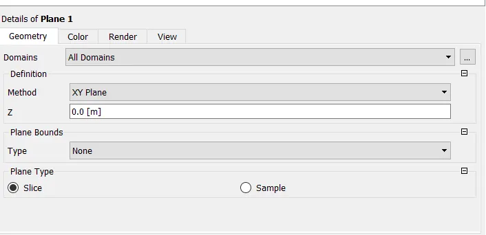
To calculate the Wall heat transfer coefficient , a plane is created in the XY plane.

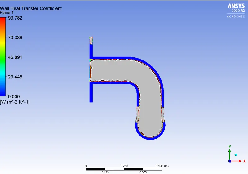
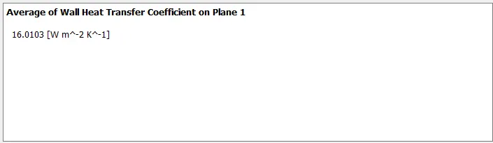
The avrage wall heat transfer coefficient at the plane created came as 16.0103 Wm^-2K^-1

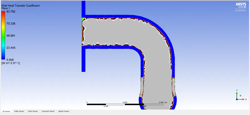
The baseline simulation gave a course mesh results. since the Wall Heat transfer coefficient is a wall phenomenon, the Wall modelling is required to capture the physics properly.

• Refined mesh with Y+ modelling:

Calculation of Reynolds number :

`Re = (rho*V*D)/(mu)`

where:

`rho`= density of the fluid.

`V`= velocity of the incoming fluid

`D`= characteristic dimension of the geometry

`mu`= viscosity of the fluid.

For this analysis ;

`rho`=1.225

`V`=5

`D`=0.17

`mu`=1.78*10^-5

`Re`=58497.19

Skin friction coefficient `Cf`=`0.079*Re^(-0.25)`

`Cf`=5.07*10^-3

Wall shear stress `Tau(w)`= `(0.5*Cf*rho*V^2)`

`Tau(w)`=0.0776

frictional velocity `u(tau)`=`((tau(w))/(rho))^(0.5)`

`u(tau)`= 0.25

`y+=(rho*u(tau)*y)/(mu)`

As the reynolds number is low, The K-Omega SST model is used for the turbukence modelling.

The y+ value falls between 10 and 30.

Considering a y+ value of 20 ; The first cell height y is obtained.

y = 1.16*10^-3 (meters)

This is the height of the centroid , So the first cell height is twice the value obtained.

first cell height = 2*(1.16*10^-3) = 2.324*10^-3 (meters)

• Meshing:

element size	0.1 meters
nodes	84459
number of elements	224154

inflation layers are added to model the y+ value .

The first cell height is 2.324 *10^-3 meters. 5 inflation layers are added , wth a growth rate of 1.2. Total thickness method is used. The geometry selection is selected as all faces in the named selection. A new named selection is created, as inflation layers.

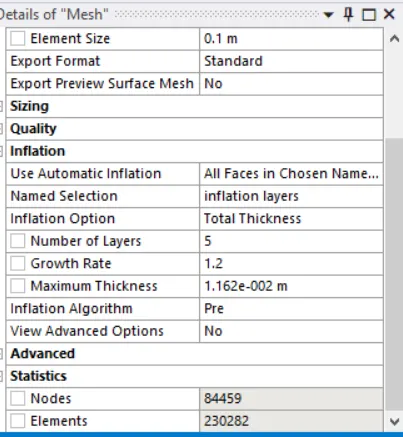
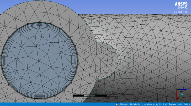
Face sizing is applied , with element size of 0.05 meters and on 11 faces

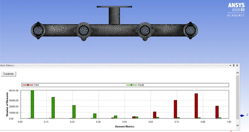
Element quality:

minimum	8.5811e-004
maximum	0.9924
average	0.46747
standard deviation	0.35042

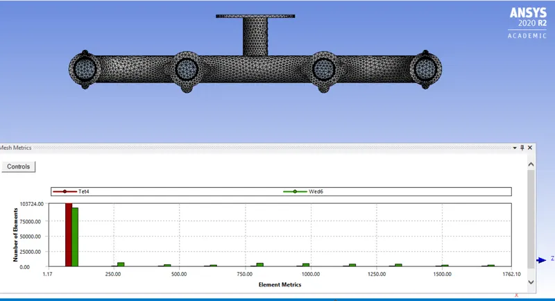
aspect ratio :

minimum	1.1745
maximum	1762.1
average	107.09
standard deviation	305.07

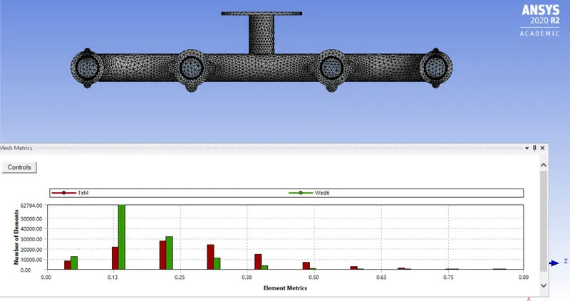
skewness:

minimum	1.3271e-003
maximum	0.8902
average	0.21399
standard deviation	0.11656

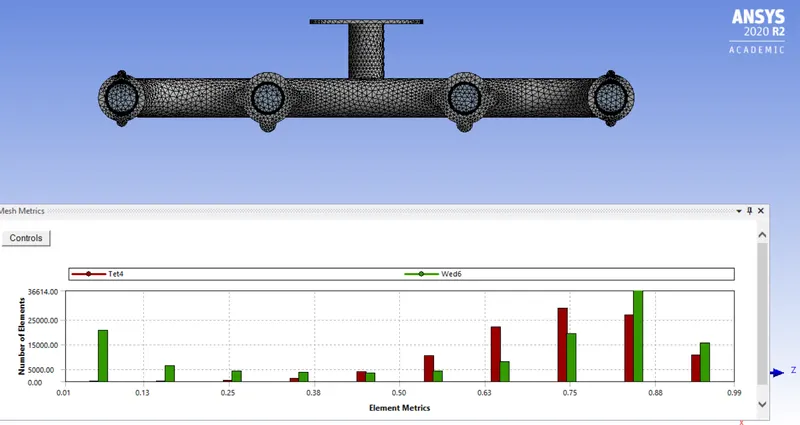
orthogonal quality:

minimum	9.38e-003
maximum	0.9903
average	0.66209
standard deviation	0.2616

• Solution:

The set up is same as the previous case

The scaled residuals, vector and the temperature contours are as follows:

• Post processing:

The wall heat transfer coefficient along the plane is obtained as:

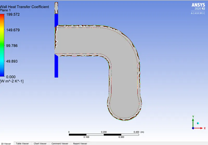
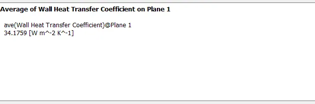
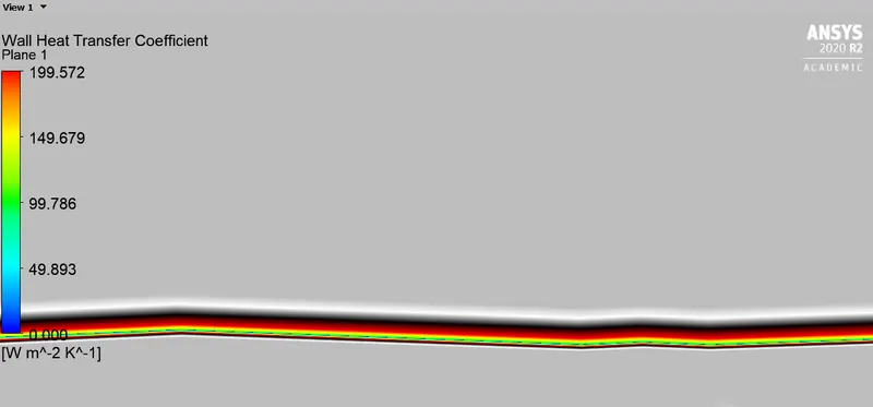
The average wall heat transfer coefficient along the plane is 34.1759 Wm^-2K^-1.

The streamlines of velocity :

The velocity distribution in the throat region is:

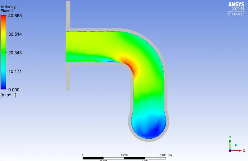
The areas where the velocity is higher, the wall heat transfer coefficient is also higher.

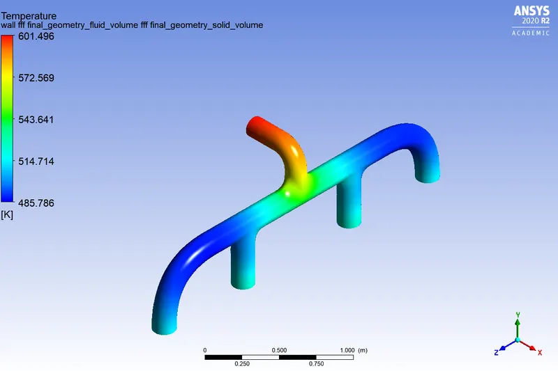
The temperature distribution in the solid body is given below:

• Analytical solution:

The emperical formula that relates to the conjugate heat transfer is given as :

`Nu=0.023*Re^0.8*Pr^0.3`

where:

`Nu`is the Nusselt number

`Pr`is the Prandtls number

Reynolds number for the analysis is calculated above as 58497.19

Nusselt number is defined as `Nu=(h*D)/k`

Prandtls number is defined as `Pr = (mu*cp)/k`

From the values of the above variable, Pr= `(1.78*10^-5*1006.43)/0.0242`

Pr=0.74

So ;

Nu = 136.83

From the expression of Nusselts number,

`h`=19.47 Wm^-2K^1

From the CFD analysis the average wall heat transfer coefficient came as 34.1759 Wm^-2K^1. The average wall heat transfer coefficient is twice the local heat transfer coefficient . The wall HTC is 34.1759/2 =17.08 Wm^-2K^-1

error = 12%

Conclusion:

The CHT analysis of an exhaust manifold is performed.

More improvements to the result obtained can be done by increasing the number of elemnts in the mesh. Due to lack of computational power , nearly 224000 elemnts are considered in this analysis. With maintaining the proper boundary conditions, and the y+ value , the wall heat transfer coefficient can be captured accurately.