Conjugate Heat Transfer Analysis on Exhaust port
AIM:
The aim of this project is to simulate conjugate heat transfer through an automobile exhaust port.
OBJECTIVES OF THE PROJECT:
- Observe the y+ value over the geometry
- Create an animation of parameters varying through the geometry
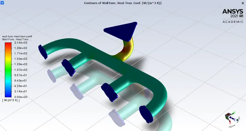
- Calculate the wall/surface heat transfer coefficient on the internal solid surface & plot the velocity & temperature contours.
THEORY:
What is Conjugate heat transfer?
Conjugate heat transfer corresponds with the combination of heat transfer in solids and heat transfer in fluids. In solids, conduction often dominates whereas, in fluids, convection usually dominates. Conjugate heat transfer is observed in many situations. For example, heat sinks are optimized to combine heat transfer by conduction in the heat sink with the convection in the surrounding fluid.
Where is CHT used?
CHT is used in designing heat exchangers, Energy Savings, Cooling of eletronic devices such as graphic cards, It can be used in places when there is a heat transfer between a solid and fluid.
In this project, we will setup conjugate heat transfer through an exhaust manifold and observe various parameters.
PROCEDURE:
SETTING UP THE CASE
Importing the geometry
For our case the geometry was already created. This is a model of an exhaust port. It can be found here.
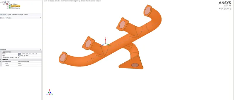
We start with importing this geometry into Ansys Fluent using the drag and drop option. For the analysis the geometry will be divided into two parts
1. Solid-Volume
2. Fluid-Volume
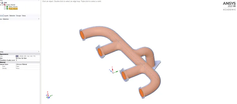
We extract these volumes using the volume extract option under prepare tab. Once these volume are extracted we add these volumes to a new component under FFF
Now we enable the share topology option under FFF. This makes sure the mesh is continuous without overlapping.
We close SpaceClaim and update the geometry on workbench.
Meshing
In the mesher, we first name the boundaries as follows,
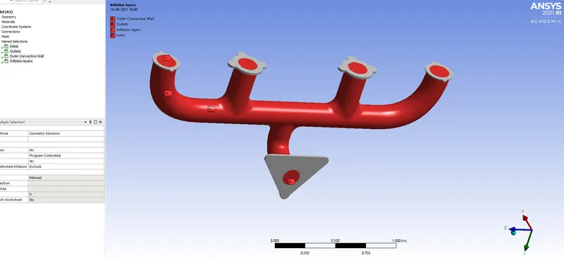
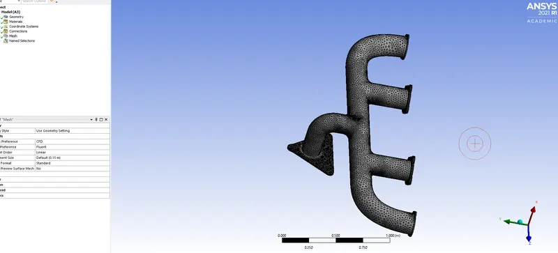
For the outer body a body-sizing option with curvature capture and for the inlets we can use an inflation layer using the total thickness method, with a thickness of 5e-3mm.
Once everything is in place the mesh should look like this
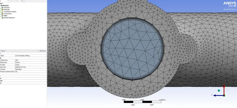
Now we export the mesh to the workbench and open the solver
In the solver, we choose a steady state, pressure based solver. We will also be slving for energy since temperature is involved.
The type of turbulence model used here is Standard K-`epsilon`model. Because K-`epsilon`models are most suitable for internal flow simulations.
Materials are
Solid - aluminium
Fluid - air
The Initial and boundary conditions are as follows,
Inlet > Velocity inlet @ 5m/s, Inlet Fluid temperature is 700k
Outlet > Pressure Outlet @ 0pa Guage pressure, Backflow outlet temperature @ 300k
Outer-Convection-wall > wall, Convective heat transfer coefficient of 20 W/(m^2)-k
Now we initialise the solution using the hybrid initialisation method and set some monitors to capture the temperature contour. We also save this animation as we capture it.
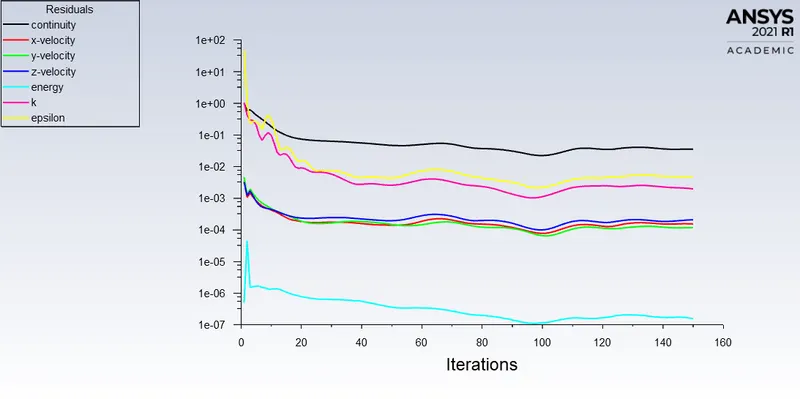
After everything is set we run the simulation for 150 iterations. Once the solution has converged we get the following results.
Residual plot
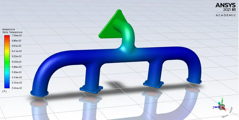
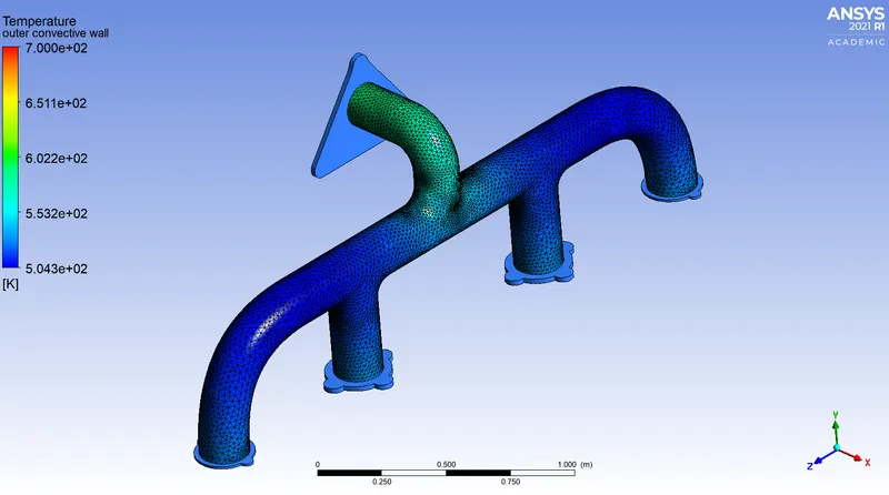
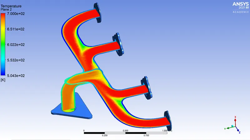
Temperature contour
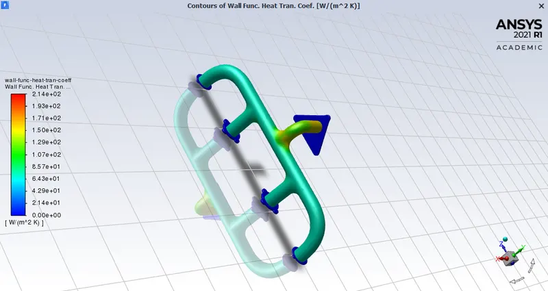
Wall heat transfer coefficient
POST-PROCESSING
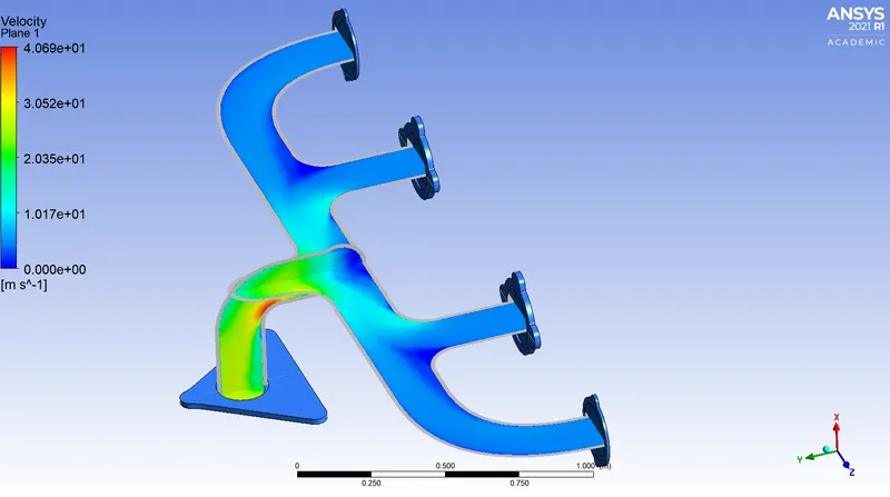
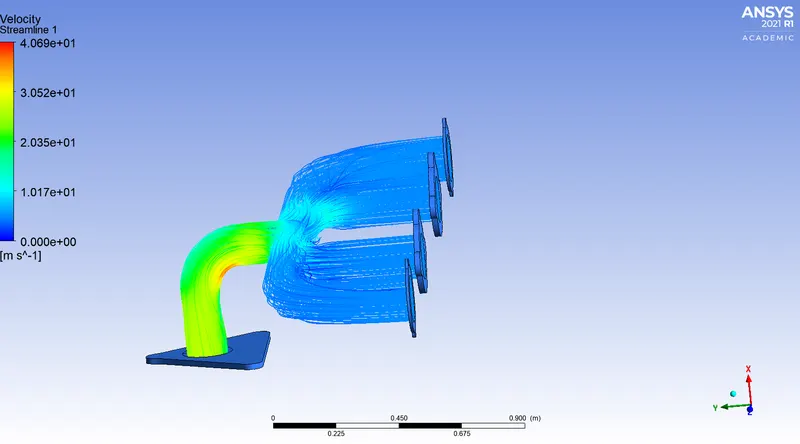
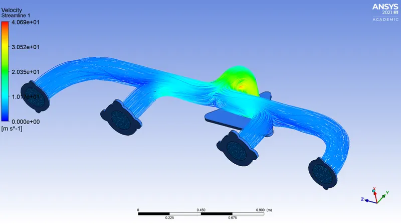
The above results are post processed using the CFD Post to get some important plots such as
Velocity Contour
Velocity Streamline plot
Temperature Contour
Verification of HTC
The results will be verified based on the numerical and graphical results. The solution must be in a physically sensible
And, If the solution is independent of the grid size then we can be sure that the solution needs no verification.
Also, the solution can be verified based on theoritical solutions. for eg, the heat transfer coefficient can also be calculated from Nusselt number
`Nu = {hL}/K`
where Nu = Nusselt number, h = HTC , K = Thermal conductivity of the solid
Nusselt number can be obtained by
`Nu = 0.23Re^{4/5}.Pr^0.3` for a flat plate.
CONCLUSION
The following conclusions have been made after observing the above plots and results
- The temperature of the pipe at the outlet has increased. This is because at the outlet all the inlets converge, therefore to conserve the mass velocity has increased. Due to the increase in velocity heat transfer due to convection has increased.
The accuracy of the prediction is depedent on
- Mesh size.
- Quality criteria such as aspect ratio of the mesh.
- Inflation layers used.
- Mesh at the solid-fluid interface.
REFERENCES