Week 4 - CHT Analysis on Exhaust port
- Give a brief description of why and where a CHT analysis is used
- Calculate the wall/surface heat transfer coefficient on the internal solid surface & show the velocity & temperature contours in appropriate areas.
- Verify if the HTC predictions from the simulations are right? On what factors does the accuracy of the prediction depend on?
Theory:
The term conjugate heat transfer is used to describe processes which involve variations of temperature within solids and fluids, due to thermal interaction between the solids and fluid.Conjugate heat transfer analysis is beneficial in accurately predicting the surface temperatures and heat exchanging capabilities of the engineering devices. Through the analysis engineers can optimize the thermal characteristics for their chosen product design.Heat transfer in solids and heat transfer in fluids are combined in the majority of applications. This is because fluids flow around solids or between solid walls, and because solids are usually immersed in a fluid. An accurate description of heat transfer modes, material properties, flow regimes, and geometrical configurations enables the analysis of temperature fields and heat transfer. Such a description is also the starting point for a numerical simulation that can be used to predict conjugate heat transfer effects or to test different configurations in order, for example, to improve thermal performances of a given application.
Typical applications of CHT are :
- HVAC
- Heat Exchanger
- Tank
- Internal Combustion Engine
- Heat Sink
- Boiler
- Reactor
- Heat Pipe
- Turbocharger
Example :
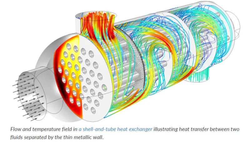
Case set up:
a) Geometry
The given model was imported to space claim .
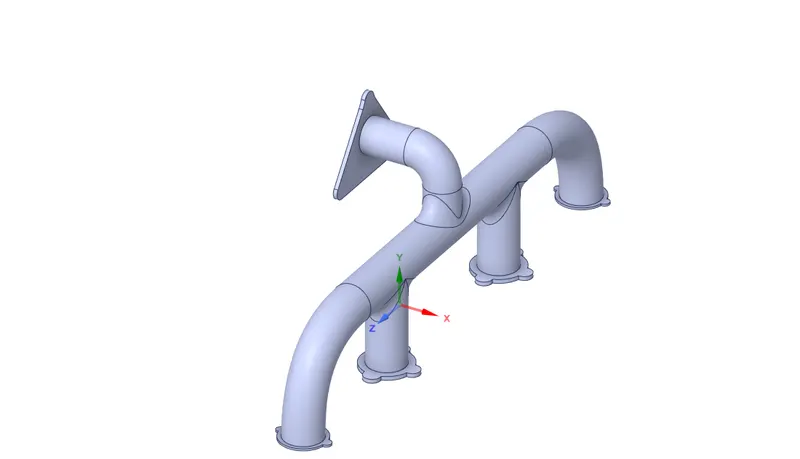
The model was checked for duplicate edges using the extra edges tool . The required fluid volume was extracted using the extract volume tool .
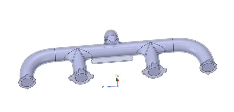
Both components were moved to a new component and Toplology was set to shared . In workbench , option was selected to share coincident topology .
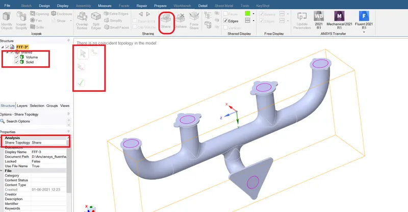
Thus geometry was set up .
Mesh:
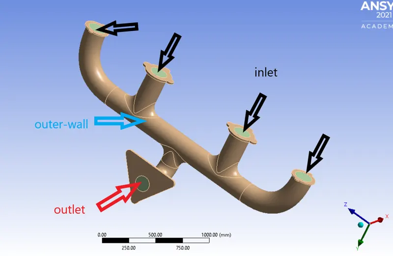
The meshing module was opened , respective faces were selected and named accordingly to mark boundaries.
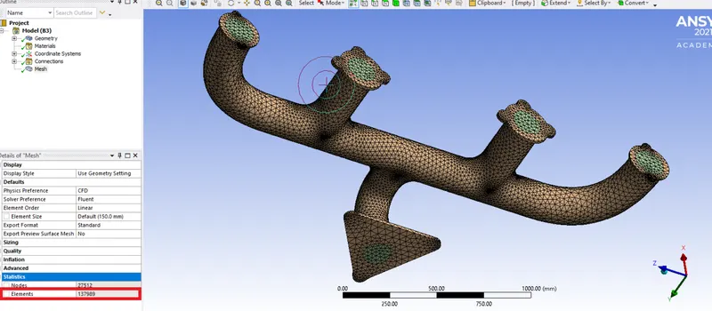
An initial mesh was generated without any refinement .
For the second case , body sizing was created , inflation layers with option to capture curvatures were generated.
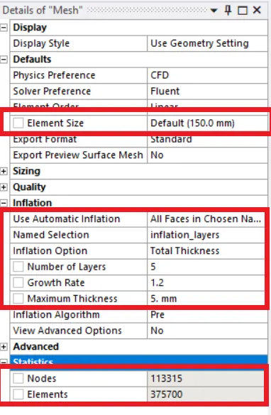
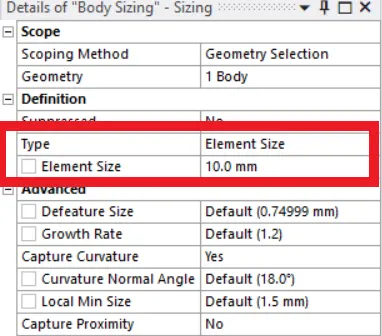
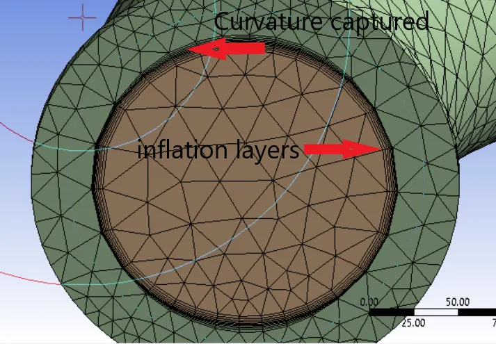
Thus meshing was completed .
Set up :
The set up module was opened with double precision and 4 core solver option.
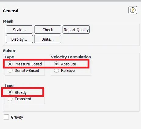
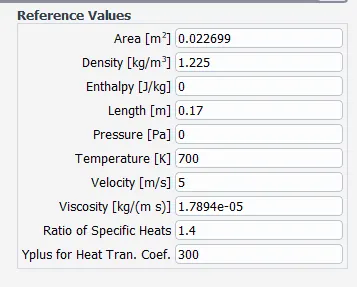
The general solver setting was used > pressure based , absolute and steady state . Respective reference values were entered.
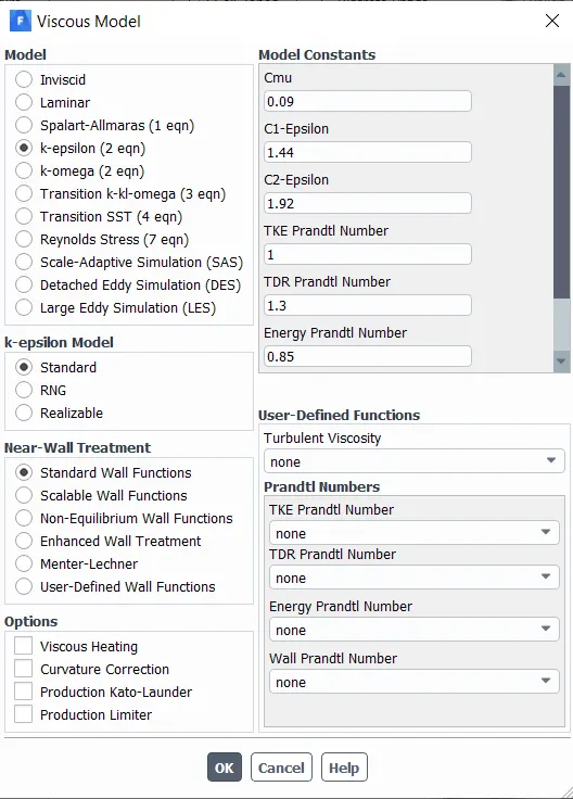
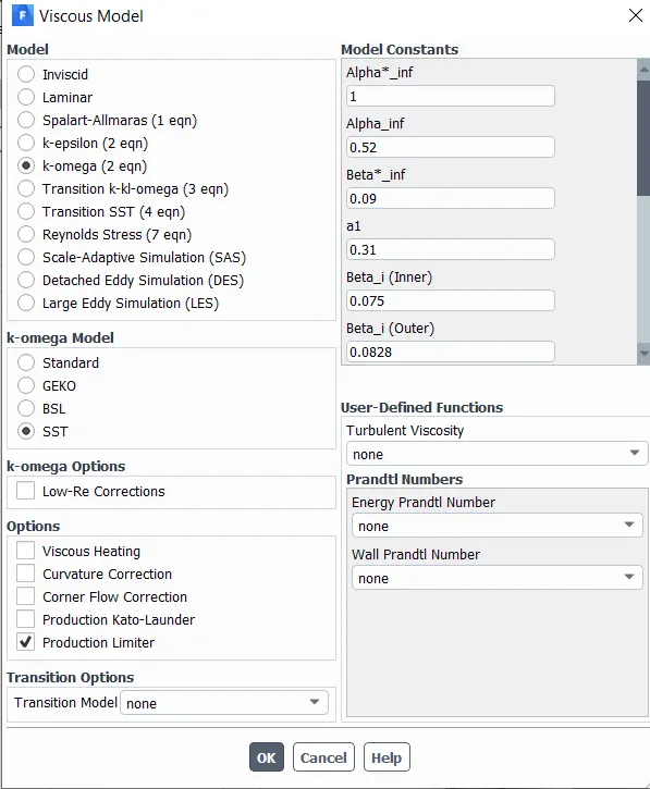
Turbulent model was set to k-epsilon for case 1 and 2 and k-omega SST for case 3 . With energy equation turned on .
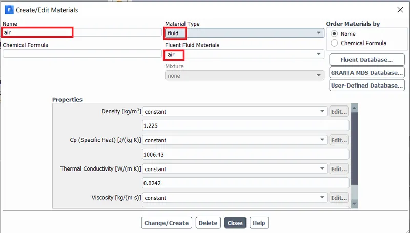
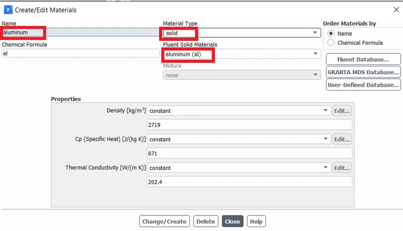
The material for fluid was set to air and solid was set to Aluminium.
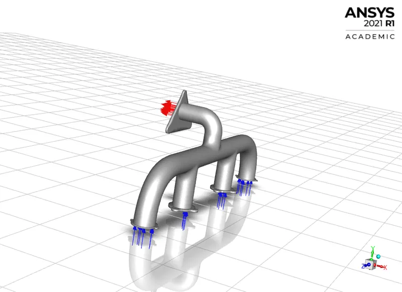
Values for various boundary conditions were entered .
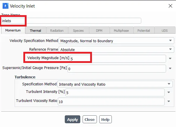
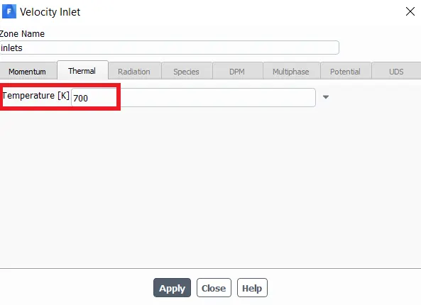
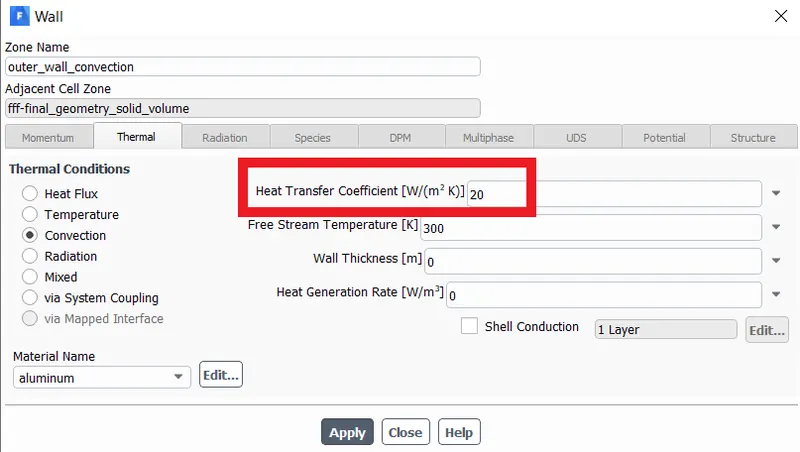
Surface report was generated to show area weighted average of surface heat transfer co-efiicient .
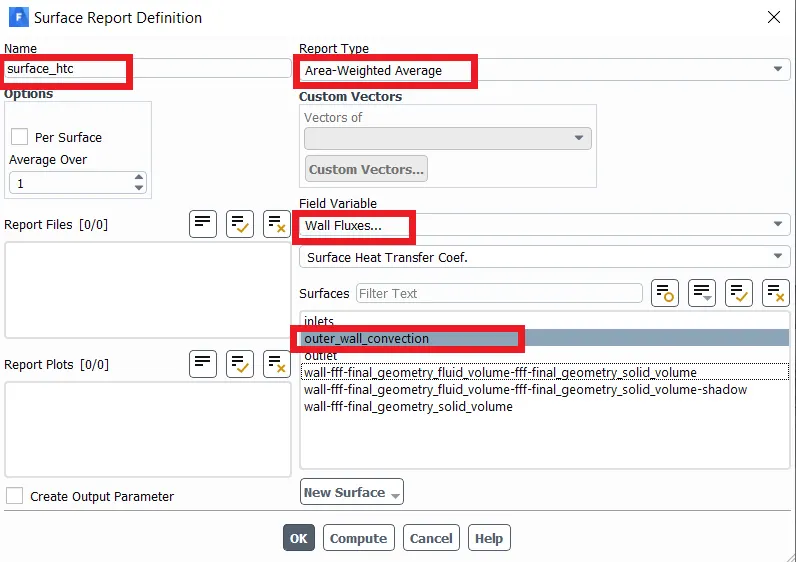
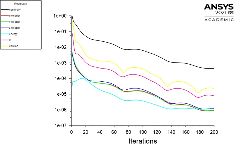
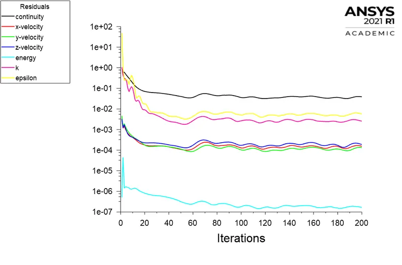
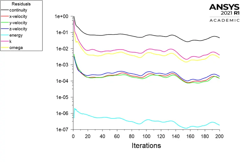
Request were made for various contours .Solution was initialized and run for 200 iterations .
Results :
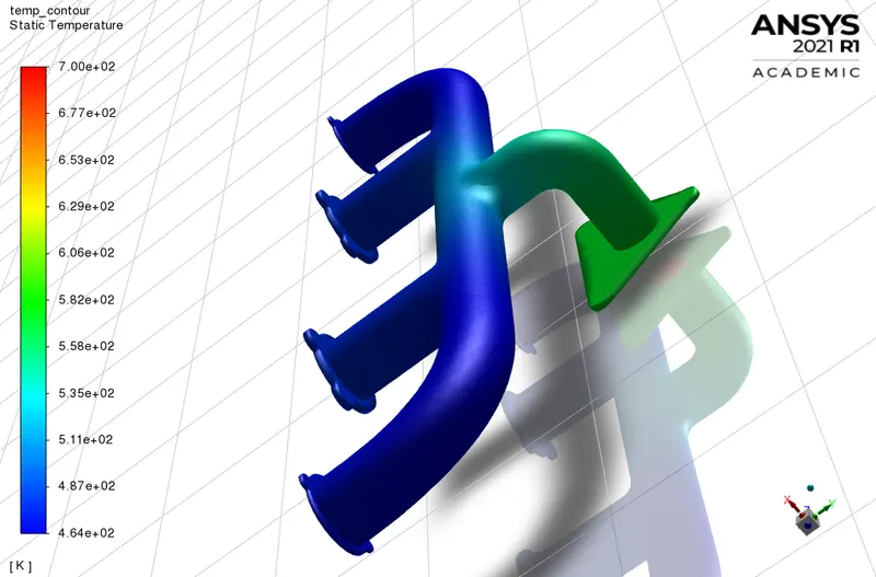
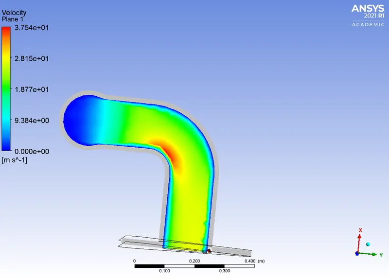
case 1 : Without mesh refinement and k-epsilon solver.
Scaled Residuals
Temperature Contour
Velocity plane
case 2 : Refined mesh and inflation layers with k-epsilon solver.
Scaled Residuals
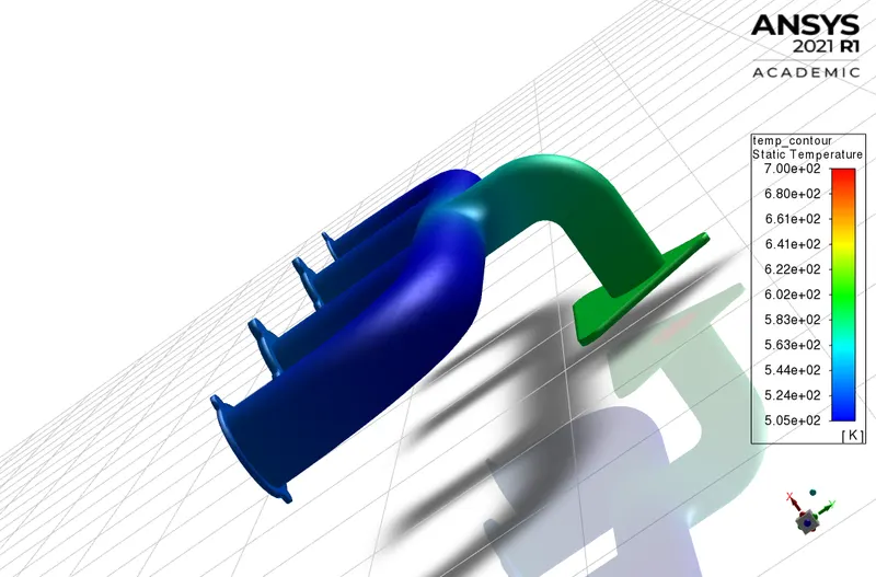
Temperature Contour
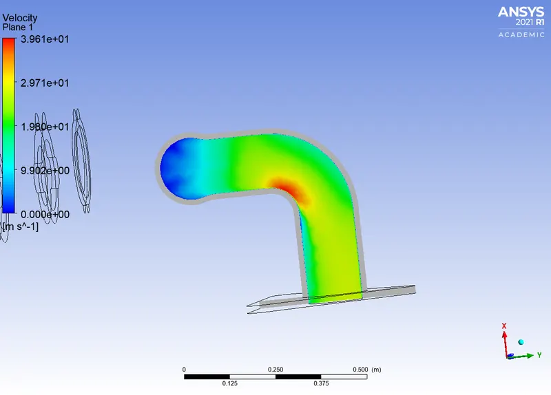
Velocity plane
case 3 :Refined mesh with K-omega SST solver .
Scaled Residuals
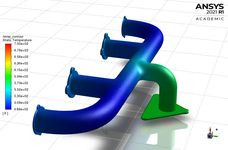
Temperature Contour
Velocity plane
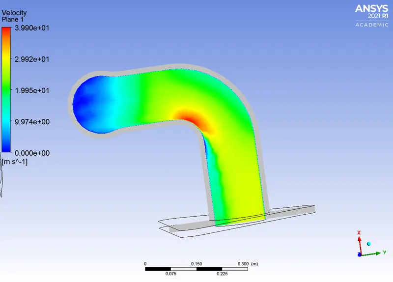
Inference:
a) There is not much difference in velocity or temperature in all the 3 cases . This implies that our baseline mesh was just as good .
b) Value for surface heat transfer co-eficient calculated for all 3 cases are listed below.
case 1: 18.633 W/m^2K
case 2: 26.799 W/m^2K
case 3: 24.344 W/m^2K
Nusselt number Nu = hD/k , where h is the heat transfer co-efficient .
Hence we can see that h is directly proportional to velocity of the fluid (since Re proportional to U). We can observe that the maximum fluid velocity is obtained at a perticular region for all 3 cases . Hence our simuations could be assumed to be good.
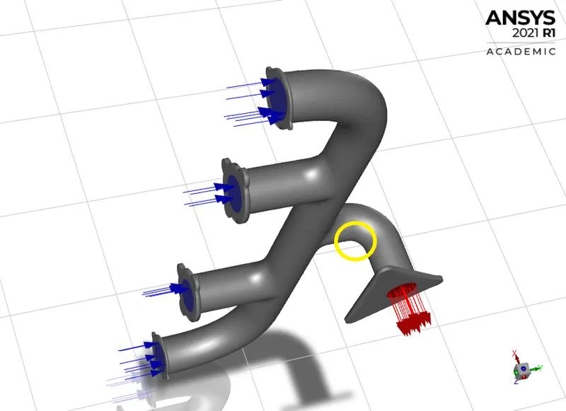
c) Factors on which accuracy depends
i) Boundary conditions provided
ii) Selection of turbulence model
iii) Mesh size as per correct y+ value.