Week 4 - CHT Analysis on Exhaust port

Aim: - To perform Conjugate Heat Transfer (CHT) Analysis on Exhaust Port of a Four Cylinder Engine.

Objective: -

1. To simulate CHT analysis on 4-cylinder engine exhaust Port.
2. To calculate wall Heat transfer Coefficient on internal wall of solid and Plot Appropriate velocity and Temperature contours.
3. To validate the Simulation And discuss CHT analysis.

Theory: -

Conjugate Heat Transfer (CHT) –

Conjugate heat transfer (CHT) analysis can accurately predict heat transfer by simultaneous solving all the relevant solid and flow field heat transfer processes.

It allows for the simulation of heat transfer between solid and fluid domains by exchanging thermal energy at the interfaces between them, which is more stable and provides faster convergence as the energy equation is strongly coupled between the solid and fluid regions.

It is preferred over Finite Element Thermal analyses for wall heat transfer coefficients and their local variations on surfaces are directly calculated within the model rather than based on simplified empirical calculations. The CHT approach therefore has benefits for those applications where heat transfer is either non-uniform or difficult to calculate empirically.

Used in Thermal analysis of –

1. Systems – HVAC, Automotive etc
2. Electronic Devices for Heat Dissipation analysis
3. Mechanical Components – Turbochargers, Combustor, Burners etc.
4. Power Plants.

Case Setup:

Geometry – Design of exhaust port is of below configuration -

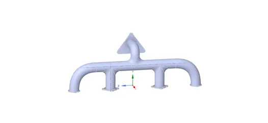
The design is prepared and the solid and fluid volume is named separately in a single component with Share Topology active so as to get conformal mesh.

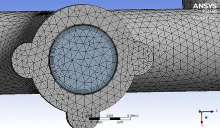
Meshing – It is done in two distinct mesh i.e., Coarser and finer mesh.

Coarser Meshing –

Number of elements – 1,37,607 Element size – 80 mm (Max. size)

No inflation layers

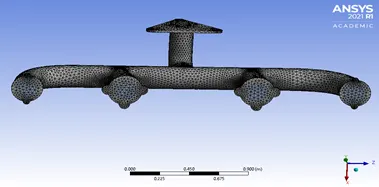
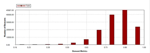
Element Metrix –

Fine Meshing –

Number of elements – 3,10,610 Element size – 20 mm (Max. size)

Number of Inflation layers – 5 (Total thickness – 10 mm)

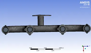
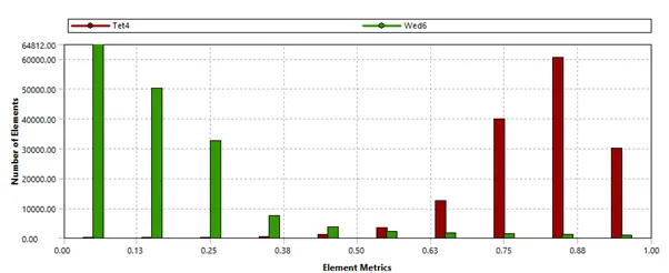
Mesh Metrix –

Y+ calculation –

First layer thickness is calculated for Y+ <= 1 is desirable for Heat Transfer calculations.

Following parameters and their values are used in calculation and case setup

Density = 1.225 kg/`m^3` Viscosity = 1.789 * 10^-5 kg/m-s Velocity at inlet =5 m/s

Average Diameter of pipe: - 166 mm

Re`= (ρ*v*l)/µ` ==> Re = 56833.4265

`C_f=0.0576/(Re)^ (1/5) ` ==> `C_f`= .0064939

`τ_w =(C_f×ρ×v^2)/2` ==> `τ_w`=.09943 N/m2

`u_f= √(τ_w/ρ)` ==> `u_f`= 0.28491 m/s

As Y+ value considered to be 1, hence first layer thickness will be –

`y=(μ*Y+)/(ρ*u_f) ` ==> y = .05125 mm

As this value is quite low and out of the capacity of the process hence y is reduced till the limit and appropriate measures such as wall function are used to minimise the error.

Solvers –

For solving above two meshes two models are used for each.

1. K-ɛ turbulence model with Enhanced Wall Treatment coupled with thermal effect Option On. As Enhanced Wall Treatment provides better results when there are two Zones/fluid bodies and reduces the dependency of Y+ or first layer’s thickness as its values are below the meshing size capacity of the processor.
2. K-ω SST (Shear Stress Transport) turbulence Model. This model provides better result at near wall region and can better capture the turbulence dissipation (turbulence kinetic energy converted into thermal internal energy) between solid and fluid common boundaries.

Note: - The energy equations are also solved for temperature, hence energy is checked.

Inputs –

Inlet velocity = 5 m/s Temperature at inlet = 700 K

Outer Solid Body – A convection medium with Heat Transfer Coefficient 20 W/m^2-K

Hybrid Initialisation is done to initialise the solution.

Results: -

1. K-ɛ model (coarser mesh) –

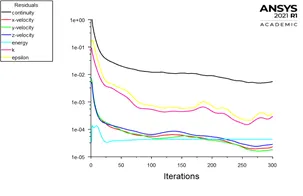
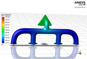
Residue plot: Temperature Contour:

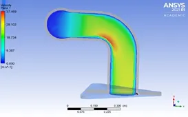
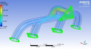
Velocity Contour and Streamline:

Inner solid wall Heat transfer Coefficient:

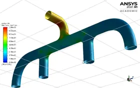
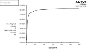
The average wall Heat transfer coefficient is 32.271 W/m^2-K.

2. K-ɛ model (finer mesh) –

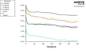
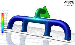
Residue plot: Temperature Plot:

Velocity Contour and Streamline:

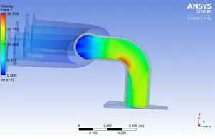
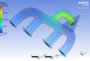
Inner solid wall Heat transfer Coefficient:

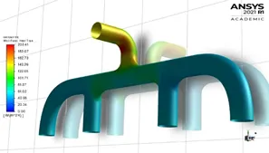
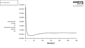
The average wall Heat transfer coefficient is 68.624 W/m^2-K

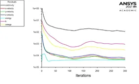
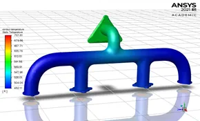
3. K-ω model (coarser mesh) –

Residue plot: Temperature Contour:

Velocity Contour and Streamline:

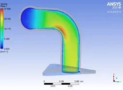
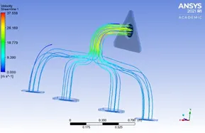
Inner solid wall Heat transfer Coefficient:

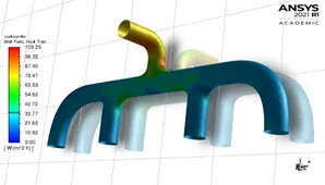
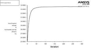
The average wall Heat transfer coefficient is 33.633 W/m^2-K

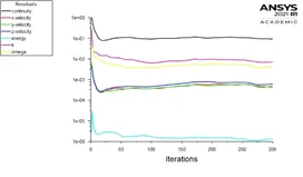
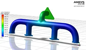
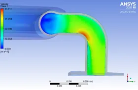
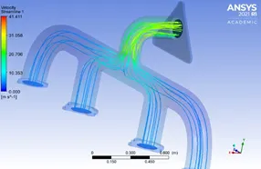
4. K-ω model (finer mesh) –

Residue plot: Temperature Plot:

Velocity Contour and Streamline:

Inner solid wall Heat transfer Coefficient:

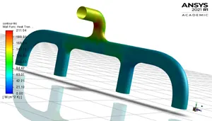
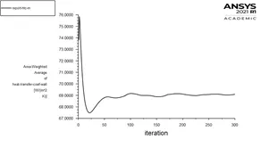
The average wall Heat transfer coefficient is 69.096 W/m^2-K

Observation Table:

Model	Number of Elements	Max. velocity (m/s)	Max. wall HTC (W/m^2-K)	Average wall HTC (W/m^2-K)
K-ɛ Turbulence Model	1,37,607	37.469	106	32.271
	3,10,610	39.670	203.41	68.624
K-ω Turbulence Model	1,37,607	37.558	109.25	33.633
	3,10,610	41.411	211.04	69.096

Validation: -

As Convective heat Transfer coefficient is a parameter to obtain Nusselt Number as –

`Nu=(h*D)/k`

also `Nu=0.023⋅Re^m⋅(Pr )^n`

And `Re=(ρ*V*D)/μ` `Pr⁡=( μ*C_p )/k`

where ρ = Density of air= 1.2 kg/m^3 μ=Dynamic viscosity (kg/m-s)

K = Thermal conductivity (w/m-k) C p = specific heat (j/kg k)

m, n are real numbers depending on condition of the flow

As velocity increases near outlet at the curve/bend due to conservation of mass flow rate, the Local Re increases as it is directly proportional to velocity. This increase In Re further increase the Nusselt Number which in turn increase the h (Convective Heat Transfer Coefficient).

As from above plots it can be observed that the location of Maximum velocity (at the curve near outlet also have high HTC are shown in red zone of the HTC contour.

Factors affecting accuracy of HTC prediction –

1. Y+ value – For heat transfer coefficient value should be less than equal to 1, or sometime less than equal to 5. If first boundary layer thickness is smaller than Viscous sublayer accuracy could be more accurate.
2. Mesh – Finer mesh give better results as compared to coarser. Mesh should be conformal and should be properly meshed at interface of the two bodies namely Fluid and solid.
3. Model – Selecting right Turbulence Model greatly impact the accuracy of results.