Week 4 - CHT Analysis on Exhaust port

AIM:

To perform the steady-state conjugate heat transfer simulation on the exhaust port when the air is coming at the inlet at a speed of 5 m/sec.

Objective:

1. Give a brief description of why and where a CHT analysis is used.
2. Maintain the y+ value according to the turbulence model and justify the results.
3. Calculate the wall/surface heat transfer coefficient on the internal solid surface & show the velocity & temperature contours in appropriate areas.
4. How would you verify if the HTC predictions from the simulations are right? On what factors does the accuracy of the prediction depend?

1. Conjugate Heat Transfer Analysis:

Conjugate heat transfer analysis is based on the mathematical structure problem, which describes the heat transfer between the body and the fluid flowing over or inside it as a result of interaction between two objects. At the matching interface, details are provided for temperature distribution and heat flux along the interface, eliminating the need to calculate the heat transfer coefficient.

The CHT analysis type allows for the simulation of the heat transfer between the solid and liquid domains by exchanging thermal energy at the interface between them. simulation of the heat exchangers, cooling of the electronic equipment, and general-purpose cooling and heating systems. In the case of the CHT that is being done in this project, we have the convection mode of heat transfer between the fluid and the solid aluminum wall of the exhaust pipe, and then the conduction mode of heat transfer is followed within the wall of the exhaust pipe.

Solving and modelling approach:

1) The exhaust pipe was modeled in the space claim.

2) The exhaust port is a three-dimensional model containing four inlets and one outlet. Despite having the isothermal boundary condition and a uniform flow rate at the four inlets, the model cannot be cut into two halves to save computational power. Therefore, the whole model needs to be discretized; this is also called space discretization.

3) CHT analysis requires both the solid and liquid volumes under consideration. Spaceclaim gives an option of volume extract for selecting the edges for fluid volume.

4) Both the solid component and the liquid component are copied into one component.

5) A shared topology is created.

6) Spaceclaim gives an option for share coincident topology when share coincident topology is selected and executed. The mesh from the fluid volume and the solid volume are said to be conformal with each other, which is a requirement for the CHT analysis.

7) The exhaust port is loaded with the proper geometry, and it is then simulated for the baseline computer-generated mesh. In the next half, we are going to use the refined mesh using the inflation layer, and the element size is to be updated to the required size, resulting in a finer result.

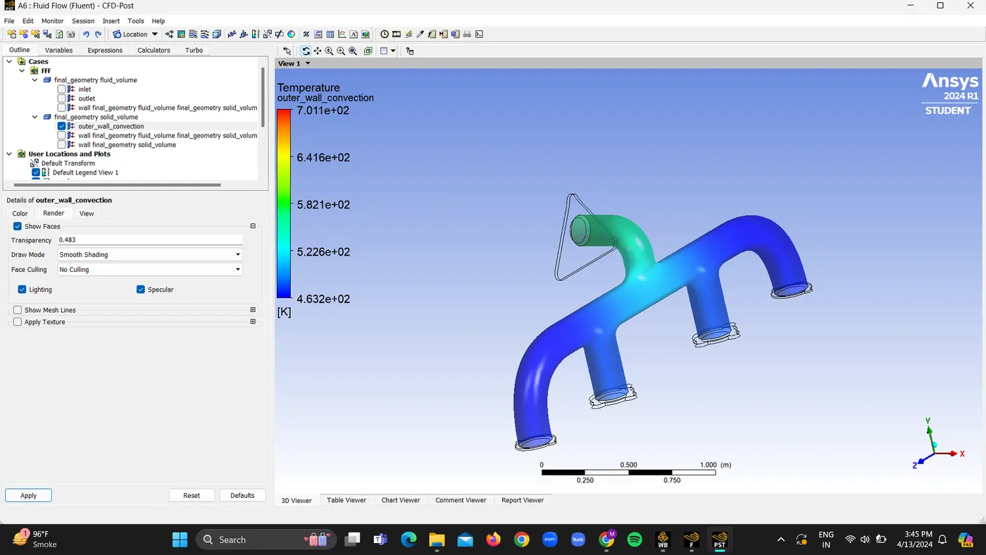
8) The named selection is created, like the inlet one, outlet one, and outlet, and the wall-convection is created to study the effect of convection from the fluid to the wall, and from the wall, the heat is dissipated by the heat conduction method.

Solving the Model and approach :

1. Geometry

2. Mehing

3. Setup

4. Solving

5. Results

A For Baseline Mesh

1. Setting up Geometry

Load the exhaust model into space claim and change the units to meters

fluid volume extraction

extraction of the fluid volume from the solid volume is what it is all about.

Share topology

Sharing data from fluid volume to solid volume is what it entails. It serves as a crucial criterion in CHT analysis.

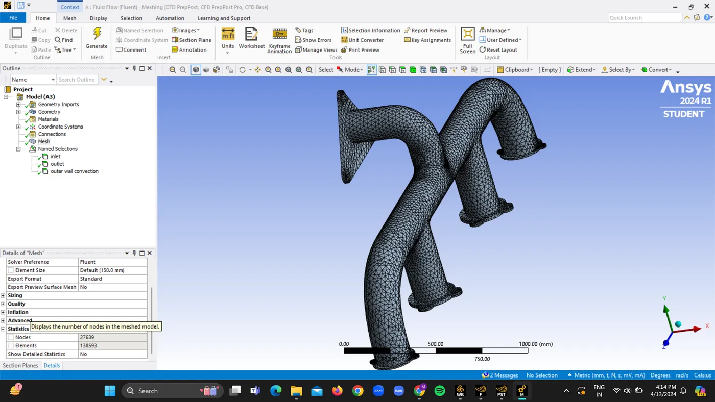
2. Meshing the Geometry :

Name the section boundaries

The default element size of ANSYS-FLUENT is used 150 mm

and generate the mesh

3. Geomtry setup :

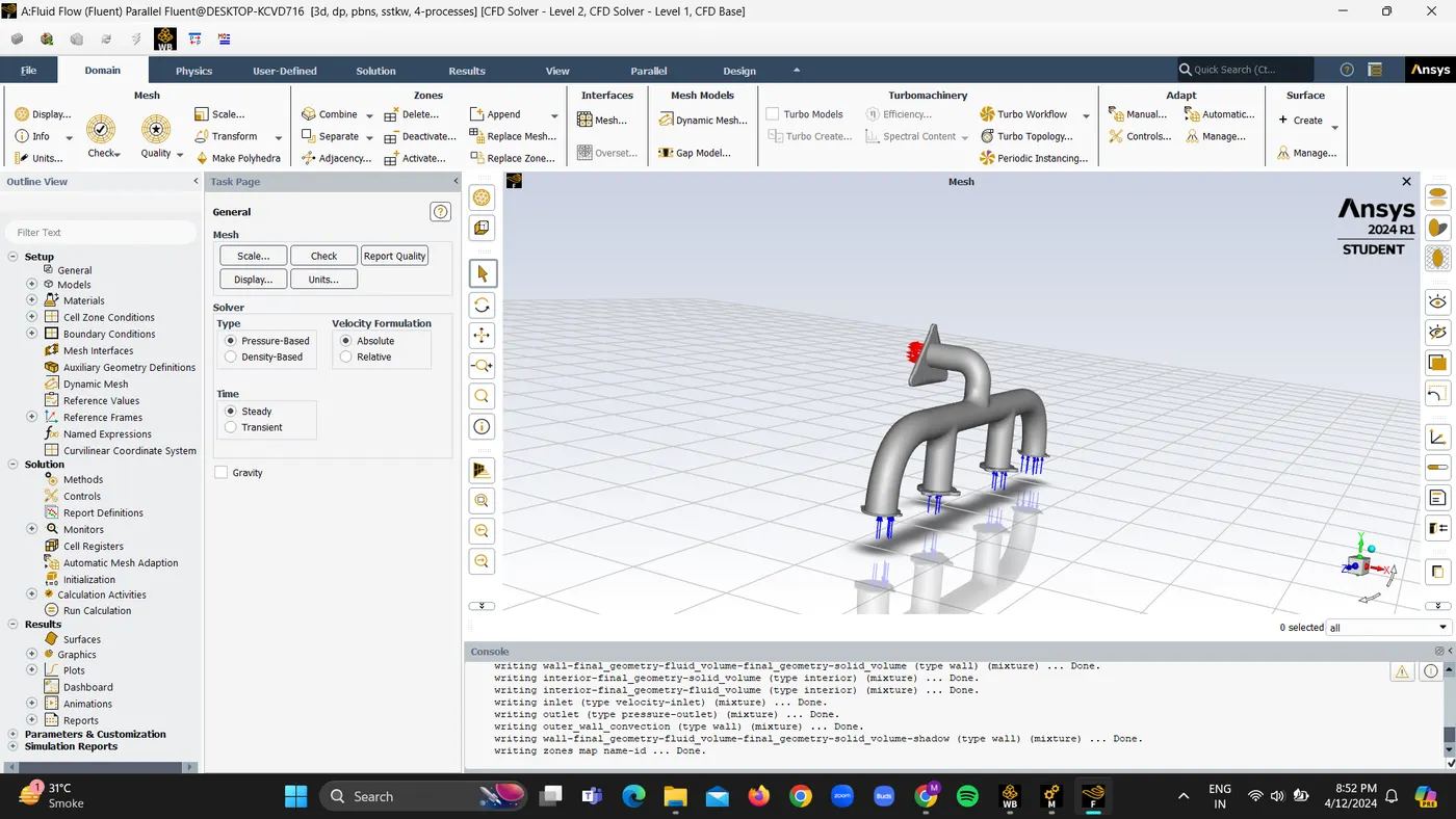
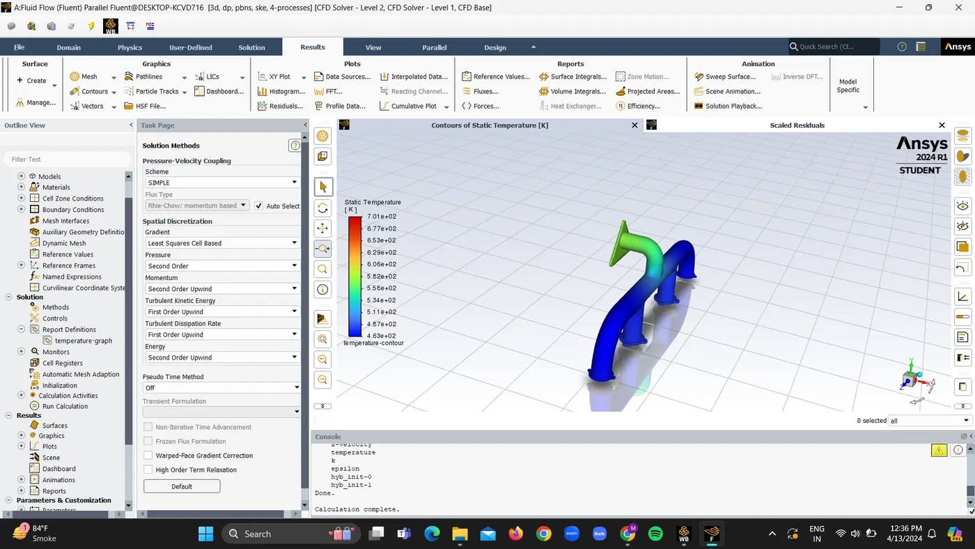
4. Solution:\

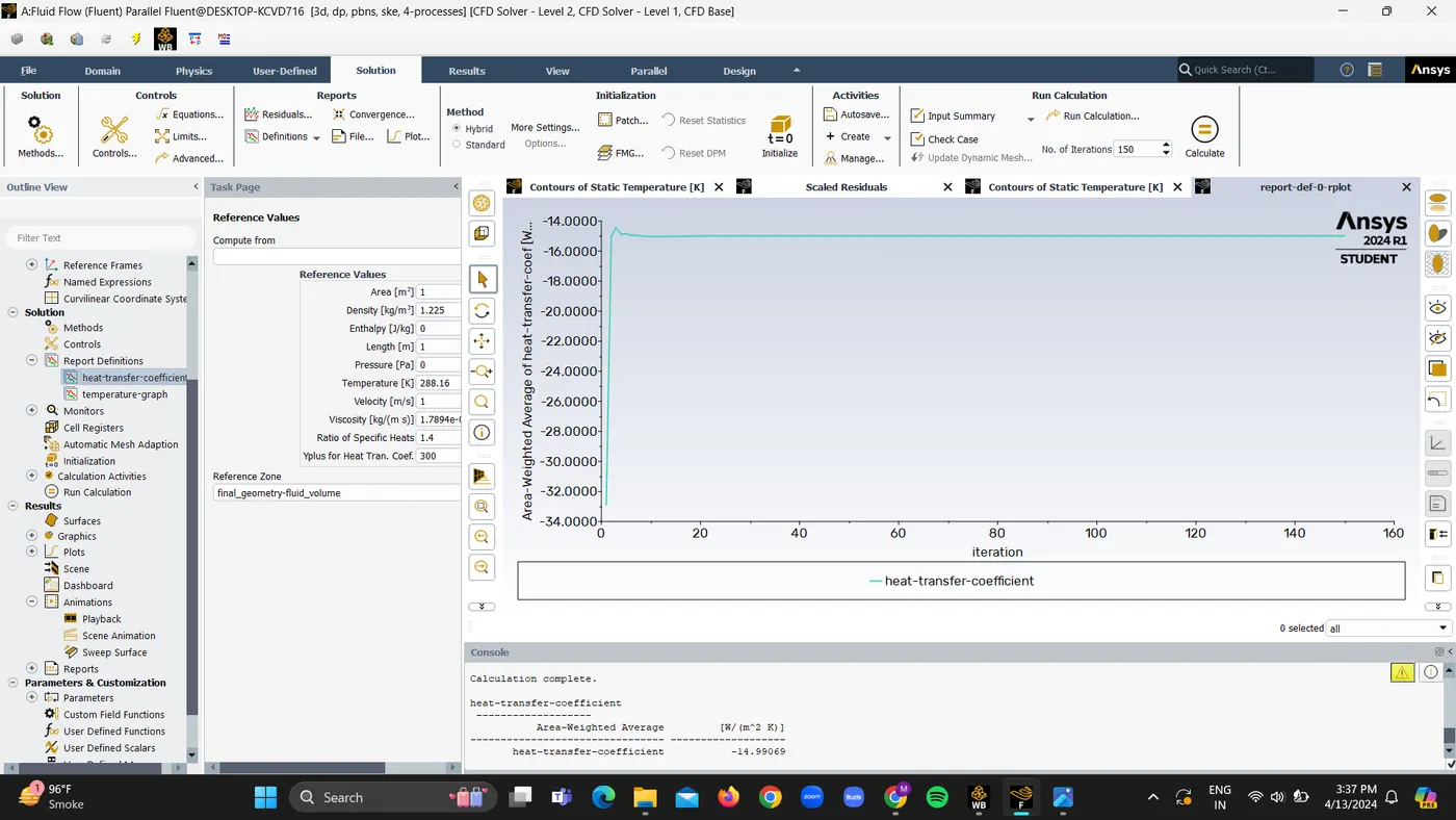
Residuals:

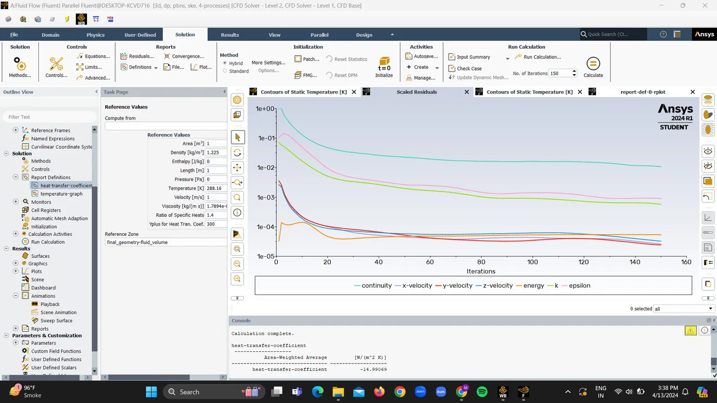
Heat tarnsfer coefficient is -14.99 W/m2K

5. Results

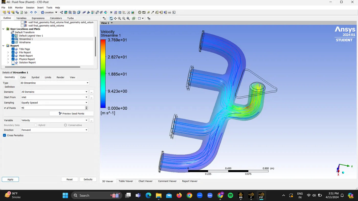
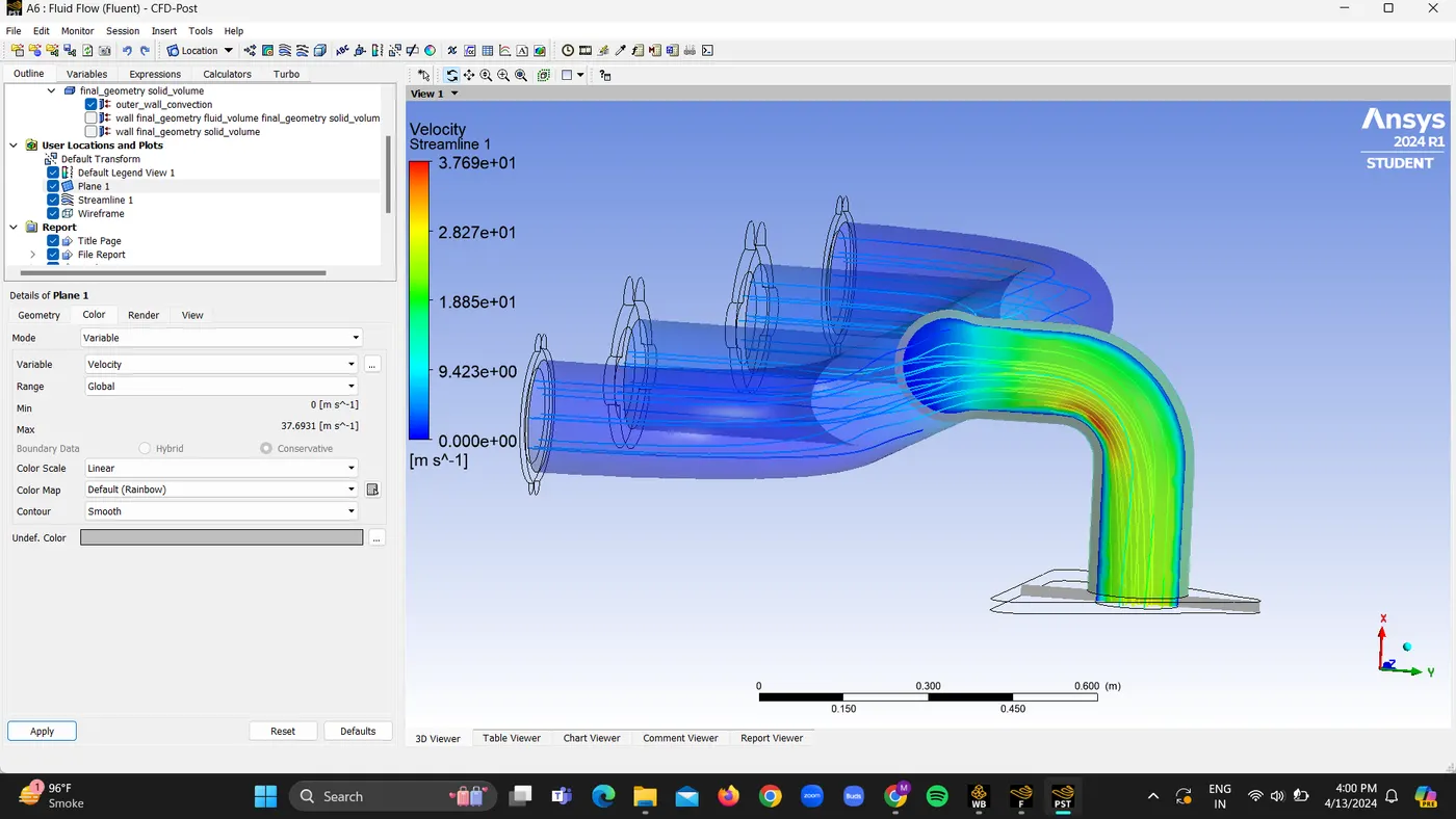
Velocity streamlines

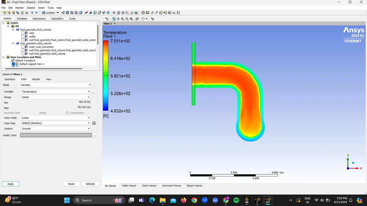
Temperature plane wrt HTC

Velocity plane wrt HTC

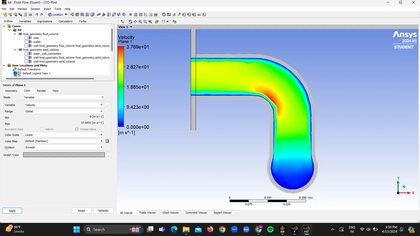
Final Result

B. For Refined Mesh

1. We need to create the inflation layers arounnd the body so to capature a good mesh with total thickness of 5mm.

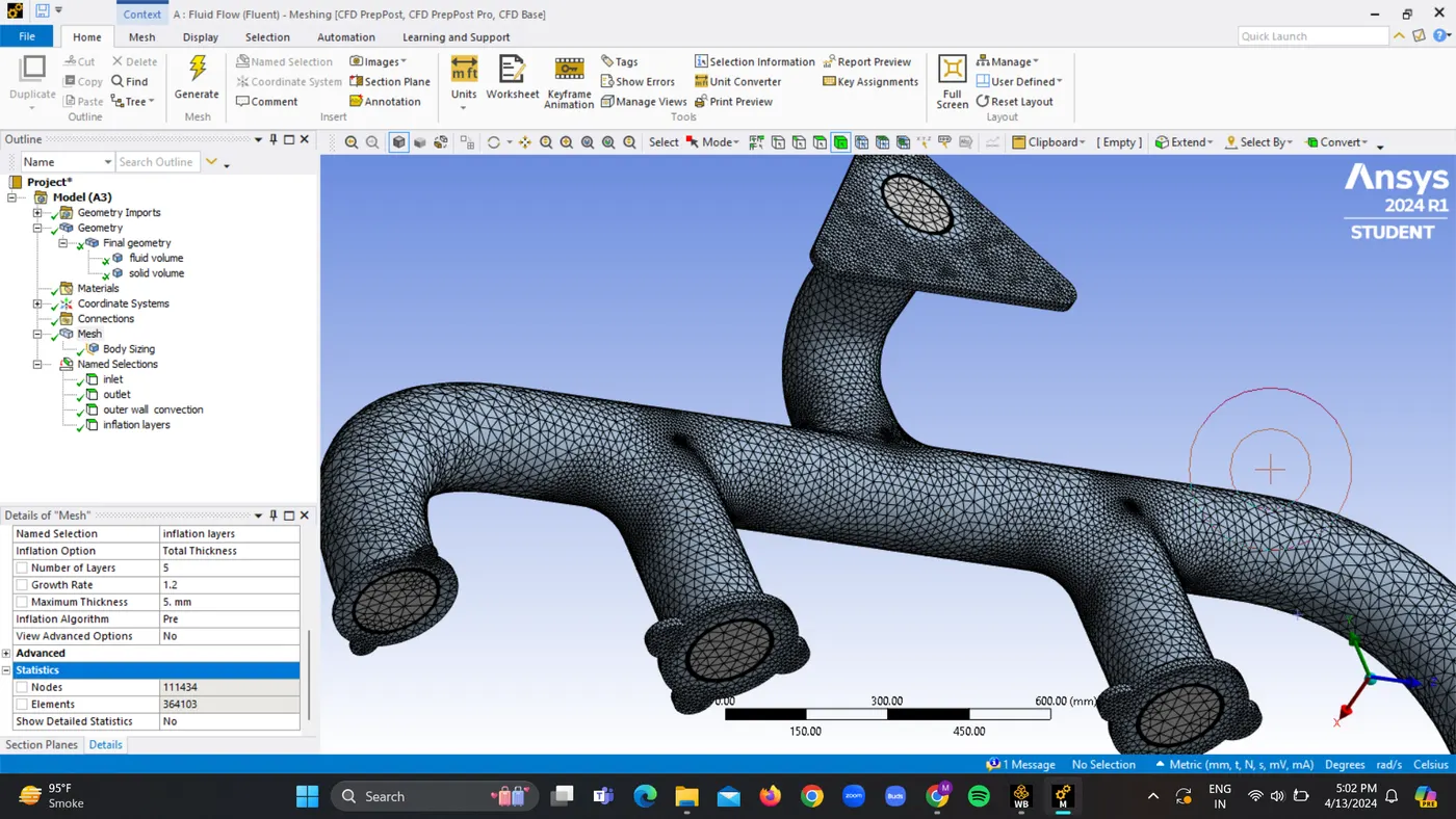
2. Then we need to create sizing and give the element size as 10 mm to capture the good mesh.

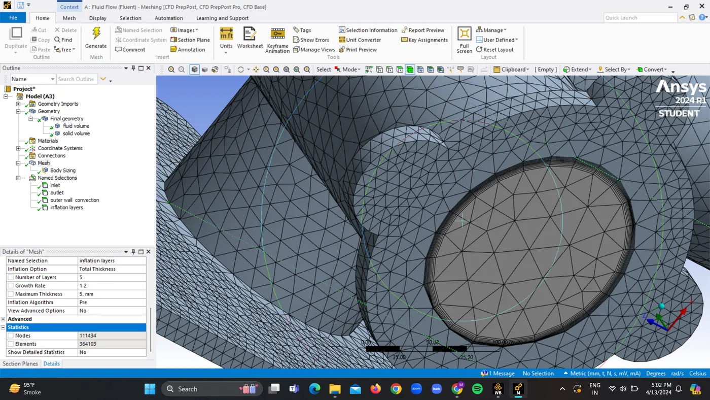
Element size is 364103

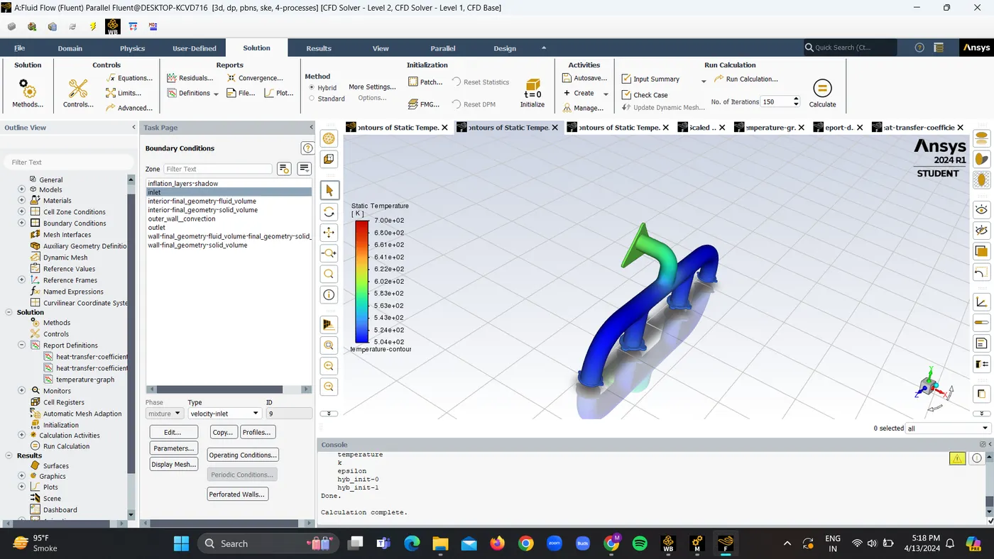
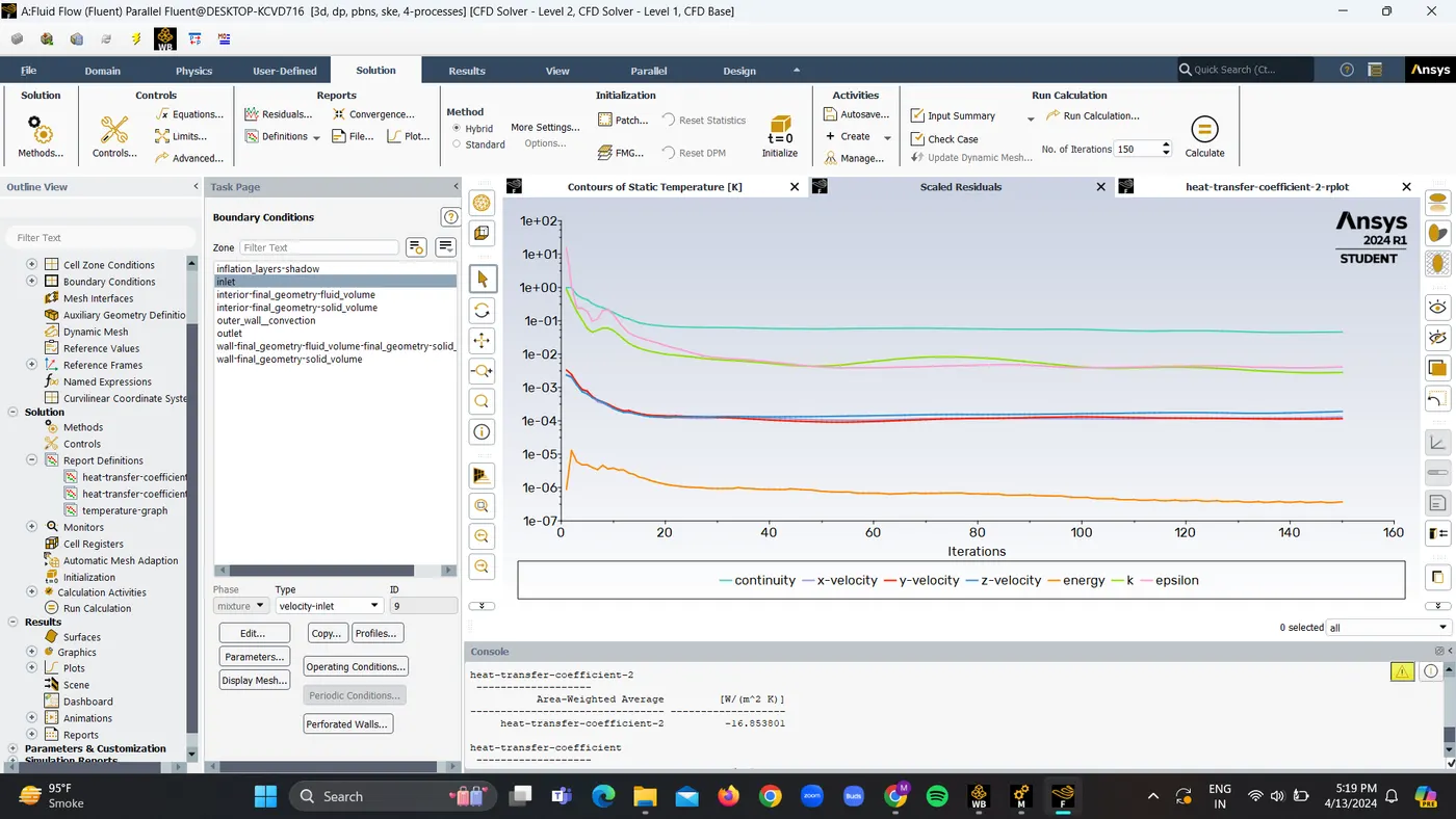
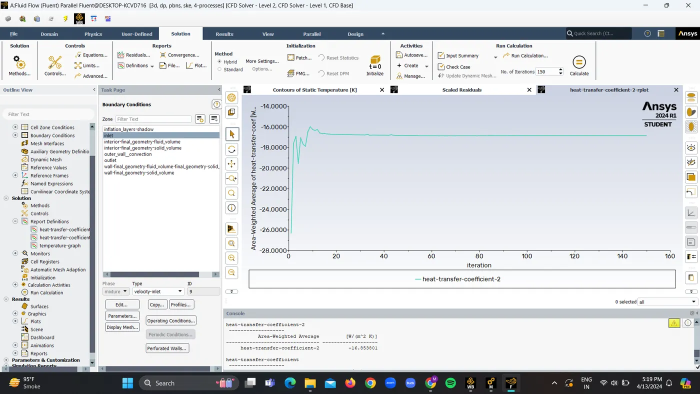
Heat Transfer coefficent for refined mesh is -16.85W/m2K

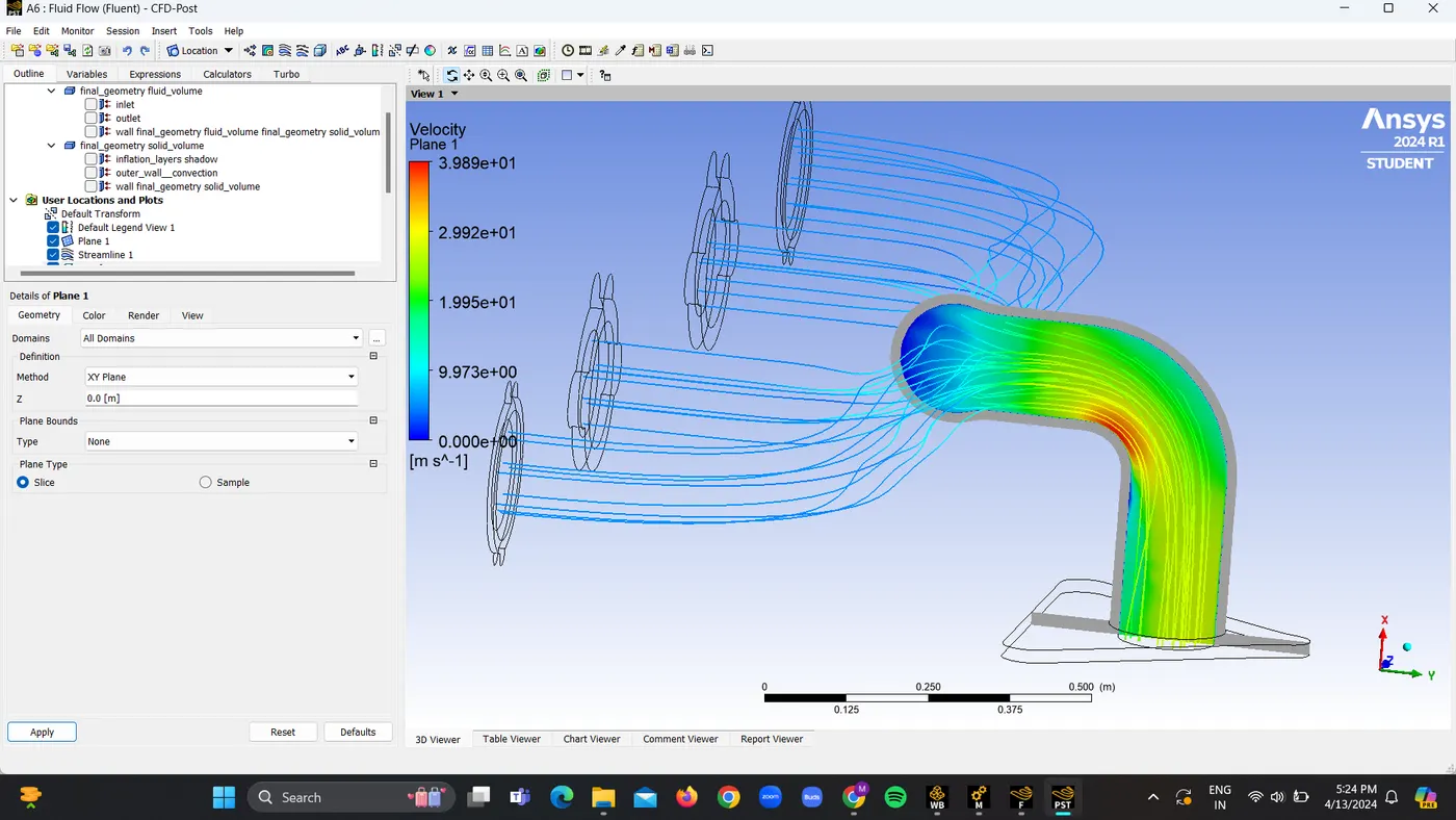
Velocity contour wrt HTC

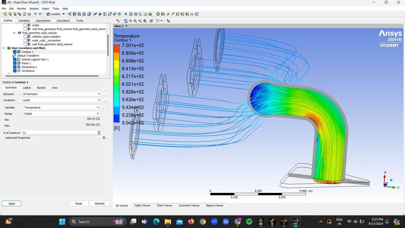
Temperature contour wrt HTC

Conclusion:

Results:

Elementsize		no of elements	HTC
150mm		138593	-14.99 W/m2K
10mm		364103	-16.85 W/m2K

we maintained Y+ value throughout inflation layer

How would you verify if the HTC predictions from the simulations are right? On what factors does the accuracy of the prediction depend on?

The typical flow conditions in automotive exhaust systems produce re in the range of 10^3 to 5*10^4. The exhaust flow often enters the region re<2300, especially in exhaust manifold runners. In spite of that, the flow remains actually turbulent since it has flowed through a substantial restriction. The exhaust valves and the persisting unsteady flow pulsation effects don’t favor the transition to the laminar region.

According to the sieder tate relation which correlates the Nu number with Re and Pr

Nu = 0.027Re^0.8Pr^1/3

It means Nusselt no. is the function of Reynolds no and Prandtl number

As the turbulent boundary layer in the bend of the outlet port is the thin maximum velocity of flow is observed at bend and hence higher Reynolds number.

Now, Nu = h*L/k

As the length of pipe and thermal conductivity is a constant value of h will increase as Nu increases and Nu increases as Re increases.

As per our result, the heat transfer coefficient is high for a higher value of velocity and hence our results are correct.

FACTORS AFFECTING THE QUALITY OF PREDICTION:

• More refined mesh leads to the better results
• Use inflation layers and apply boundary conditions
• Proper selection of turbulence model according to Y+ values.
• Using ANSYS-FLUENT, the CHT analysis of the exhaust port was successfully simulated.
• The entire geometry is discretized using a pressure-based, coupled scheme solver.
• We can select the value of Y + = 1 (viscous sublayer) and the turbulent model k S S T because the heat transfer coefficient value is found in the cell next to the wall.

in this study, CHT analysis has done to find temperature rise at the manifold because of hot air passing through it and we predicted the heat transfer coefficient, as well as velocity contours, were created to get insight into the fluid path and maximum velocity area.

It is found that the heat transfer coefficient is more near the wall where the exhaust pipe bends.

Higher the velocity higher will be the Heat Transfer Coefficient with higher heat temperature.