Week 4 - CHT Analysis on Exhaust port

Aim 

To perform the steady-state conjugate heat transfer simulation on the exhaust port when the air is coming at the inlet at a speed of 5m/sec.

1. Give a brief description of why and where a CHT analysis is used.?

Conjugate Heat Transfer (CHT) analysis is a computational technique used to simulate the simultaneous heat transfer processes occurring in both solid structures and surrounding fluids. This type of analysis is employed when there is a significant interaction between the heat transfer phenomena in a solid material and the adjacent fluid, such as in situations involving fluid flow over heated surfaces, cooling of electronic components, or heat exchangers.

CHT analysis is particularly useful in scenarios where accurate prediction of temperature distributions and heat transfer rates is crucial. Some common applications include:

1. Aerospace and Automotive Industries: CHT analysis is employed to study the thermal behaviour of aircraft engine components, like turbine blades, where high-temperature fluid flows interact with solid structures. In the automotive sector, it is used to model cooling systems and predict engine performance.
2. Electronics Cooling: For electronic devices like computer chips or circuit boards, CHT analysis helps engineers ensure proper cooling to prevent overheating and maintain optimal operating conditions.
3. Energy Systems: Conjugate heat transfer is utilized in designing and optimizing energy systems, such as nuclear reactors or power plants, where efficient heat transfer between the reactor core and coolant is crucial.

Simulation procedure:

We are going to simulate the exhaust port refine mesh

Geometry:

1. Import the model of exhaust port.

2. Go in repair and clear the extra edges if any.

3. Then go in prepare and extract the inner volume.

4. After that select solid and fluid component move them to new component.

5. Finally go in workbench and select share prep and share the topology in meshing.

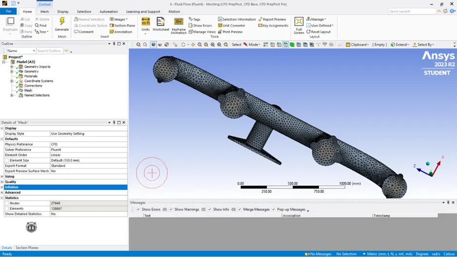
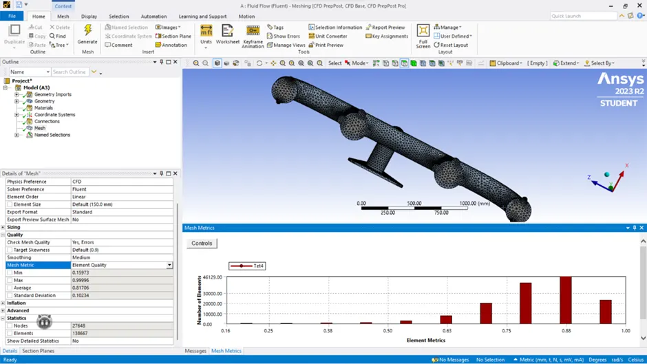
Mesh:

• Open the mesh section in workbench.
• First name the faces which are inlets, outlet, outer-wall-convection.
• Then mesh the geometry as default mesh size.
• Then we can add the inflation layer so, can get the better result in the wall surface. 

Total layer thickness =5mm

Maximum layer = 6

Growth rate = 1.2

 

Setup:

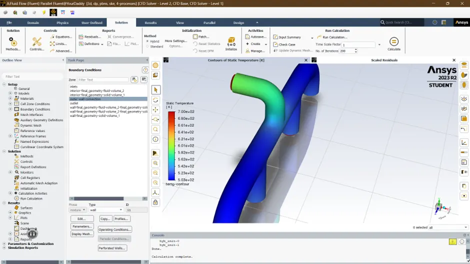
• Turn on the energy equation and viscous model.
• Set up the materials, solid and fluid one.
• Then set up the boundary conditions like inlet velocity, outlet pressure, outer wall convection's HTC.
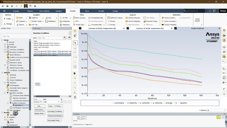
• initialize the solution
• add the contour plot

Inlet-velocity-5 m/s

Temperature- 700°C

Outlet-Gauge pressure- 0 pa

Outer wall convection

wall heat transfer co-efficient (h)= 20k

 

 

 

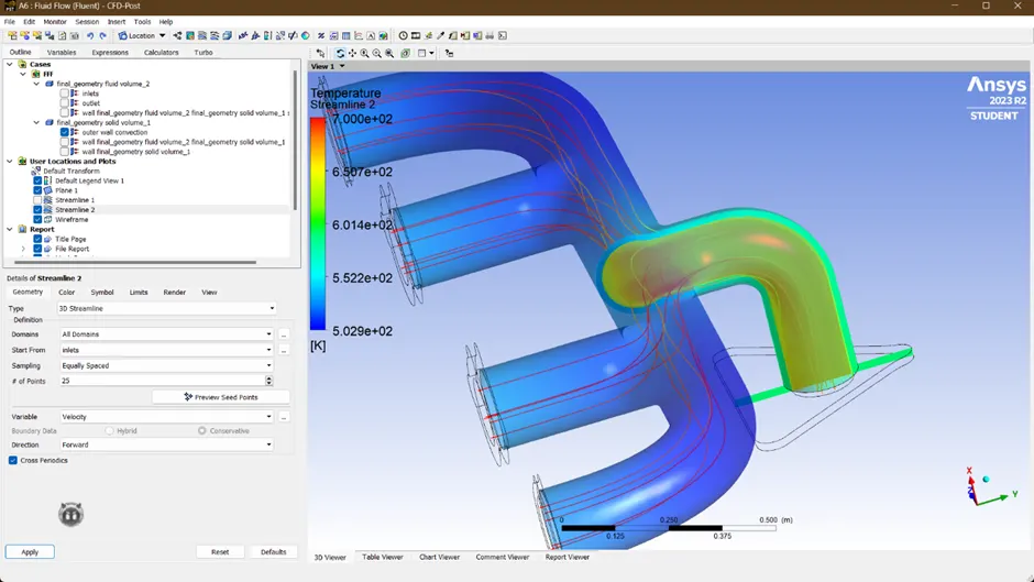
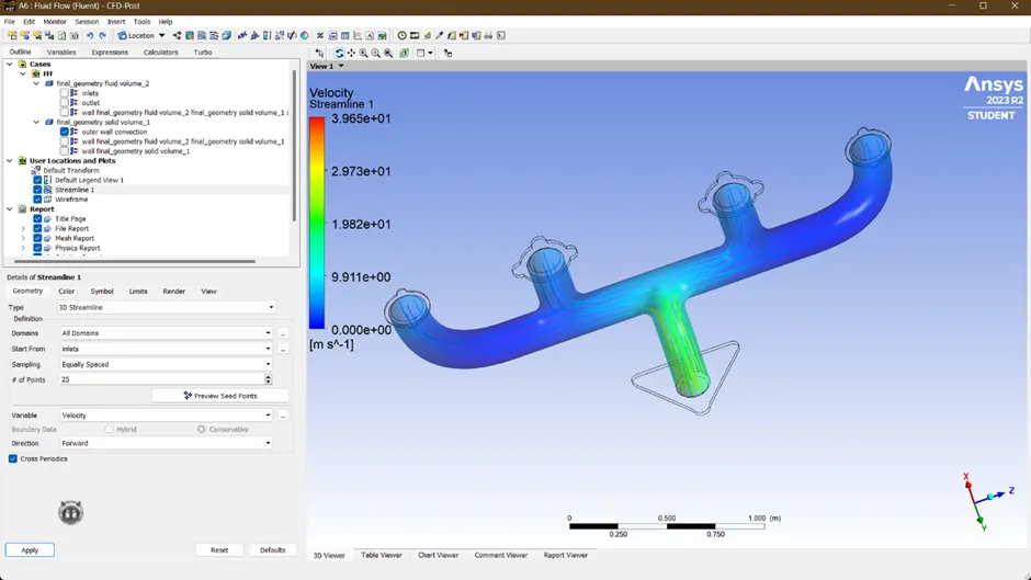
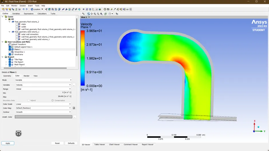
How would you verify if the HTC predictions from the simulations are right? On what factors does the accuracy of the prediction depend on?

The typical flow conditions in automotive exhaust systems produce re in the range of 10^3 to 5*10^4. The exhaust flow often enters the region re<2300>

According to the sieder tate relation which correlates the Nu number with Re and Pr

Nu = 0.023*Re^0.8Pr^n

It means Nusselt no. is the function of Reynolds no and Prandtl number

As the turbulent boundary layer in the bend of the outlet port is the thin maximum velocity of flow is observed at bend and hence higher Reynolds number.

Now, Nu = h*L/k

As the length of pipe and thermal conductivity is a constant, value of h will increase as Nu increases and Nu increases as Re increases.

As per our result, the heat transfer coefficient is high for a higher value of velocity and hence our results are correct.

Re=Density*velocity*length/dynamic viscosity

Re=1.225*5*0.166/1.789e^-5

Re = 0.5683

By using the Dittus Bolter heat transfer coefficient relation in natural turbulent flow the Diltus Bolter HT coefficient is determined by the Nusselt number which is related by the formula of 

Nu(D) = 0.023* Re^0.8*pr^n

Here, n=0.3, D= diameter of the pipe= characteristics length = 0.166 m

Prandtl number

pr = mu*cp/k   

here mu= 1.789*10^-5, cp = 1006.43 J/kg-k and k = thermal conductivity = 0.2556 w/mk

pr = (1.789*10^-5*20)/0.2556 

pr= 7.156

Nusselt number is calculated as

NU = 0.023*0.5683^0.8*7.156^0.3

NU= 32.4726

Nu= h*L/k => 32.4726= h*0.166/0.2556

H= 49.99w/m^2k

Conclusions-

Here we find the theoretical value and the computational value of the thermal specific heat transfer coefficient to be= 49.99. so, the value is high to the value of h in the computational way which is = 20 w/m^2k.

The velocity at the outlet is high than in the inlet this can be attributed to one outlet and the four inlets.

For further proceedings the mesh should be fine and y+ should compatible with it.