Challenge

Week 4 - CHT Analysis on Exhaust port

BBaskar Ayyakkannu7 Jun 2023

AIM:

To simulate the Conjugate Heat Transfer Analysis on exhaust port using ansys fluent.

OBJECTIVES:

Give a brief description of why and where a CHT analysis is used.
Maintain the y+ value according to the turbulence model and justify the results.
Calculate the wall/surface heat transfer coefficient on the internal solid surface & show the velocity & temperature contours in appropriate areas.
How would you verify if the HTC predictions from the simulations are right? On what factors does the accuracy of the prediction depend on.

CONJUGATE HEAT TRANSFER(CHT):

The Conjugate Heat Transfer (CHT) analysis type allows heat transfer simulation between solid and fluid domains by exchanging thermal energy at the interference between them.

Conjugate Heat Transfer analysis allows for the simulation of heat transfer between solid and fluid domains by exchanging thermal energy at the interfaces between them and transporting via conduction within solids and additionally via convection within fluid domains. Conjugate heat transfer analysis can accurately predict heat transfer by solving all the relevant solid and flow field heat transfer processes simultaneously.

How is Heat Transferred:

Heat can travel from one place to another in several ways. The different modes of heat transfer include:

Conduction
Convection
Radiation

Meanwhile, if the temperature difference exists between the two systems, heat will find a way to transfer from the higher to the lower system.

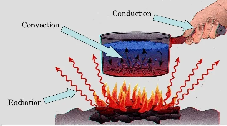
Conduction:

Conduction is defined as

The process of transmission of energy from one particle of the medium to another with the particles being in direct contact with each other.

An area of higher kinetic energy transfers thermal energy toward the lower kinetic energy area. High-speed particles clash with particles moving at a slow speed, as a result, slow-speed particles increase their kinetic energy. This is a typical form of heat transfer and takes place through physical contact. Conduction is also known as thermal conduction or heat conduction.

Conduction Equation

The rate of conduction can be calculated by the following equation,

`Q=(K.A.(T_(hot)-T_(cold)))/d`

Where,

Q is the transfer of heat per unit of time
K is the thermal conductivity of the body
A is the area of heat transfer
T_hot is the temperature of the hot region
T_cold is the temperature of the cold region
d is the thickness of the body

The coefficient of thermal conductivity shows that a metal body conducts heat better when it comes to conduction.

Conduction Examples

Following are the examples of conduction:

Ironing of clothes is an example of conduction where the heat is conducted from the iron to the clothes.
Heat is transferred from hands to ice cube resulting in the melting of an ice cube when held in hands.
Heat conduction through the sand at the beaches. This can be experienced during summers. Sand is a good conductor of heat.

Convection:

Convection is defined as

The movement of fluid molecules from higher temperature regions to lower temperature regions.

Convection Equation

As the temperature of the liquid increases, the liquid’s volume also has to increase by the same factor and this effect is known as displacement. The equation to calculate the rate of convection is as follows,

`Q = h_c *A*(T_s -T_f)`

Where,

Q is the heat transferred per unit of time
h_c is the coefficient of convective heat transfer
A is the area of heat transfer
T_s is the surface temperature
T_f is the fluid temperature

Convection Examples

Examples of convection include:

Boiling of water, that is molecules that are denser move at the bottom while the molecules which are less dense move upwards resulting in the circular motion of the molecules so that water gets heated.
Warm water around the equator moves towards the poles while cooler water at the poles moves towards the equator.
Blood circulation in warm-blooded animals takes place with the help of convection, thereby regulating the body temperature.

Radiation:

Radiant heat is present in some other form in our daily lives. Thermal radiation are referred to as radiant heat. Thermal radiation is generated by the emission of electromagnetic waves. These waves carry away the energy from the emitting body. Radiation takes place through a vacuum or transparent medium which can be either solid or liquid. Thermal radiation is the result of the random motion of molecules in matter. The movement of charged electrons and protons is responsible for the emission of electromagnetic radiation. Let us know more about radiation heat transfer.

Radiation heat transfer is measured by a device known as a thermocouple. A thermocouple is used for measuring the temperature. In this device sometimes, error takes place while measuring the temperature through radiation heat transfer.

Radiation Equation

As temperature rises, the wavelength in the spectra of the radiation emitted decreases and shorter wavelengths of radiations are emitted. Thermal radiation can be calculated by Stefan-Boltzmann law,

`P = e ∙ σ ∙ A· (Tr – Tc)4`

Where,

P is the net power of radiation
A is the area of radiation
Tr is the radiator temperature
Tc is the surrounding temperature
e is emissivity and σ is Stefan’s constant (σ = 5.67 × 10^-8Wm^-2K^-4

Radiation Example

Following are the examples of radiation:

Microwave radiation emitted in the oven is an example of radiation.
UV rays coming from the sun is an example of radiation.
The release of alpha particles during the decaying of Uranium-238 into Thorium-234 is an example of radiation.

SPACECLAIM SETUP:

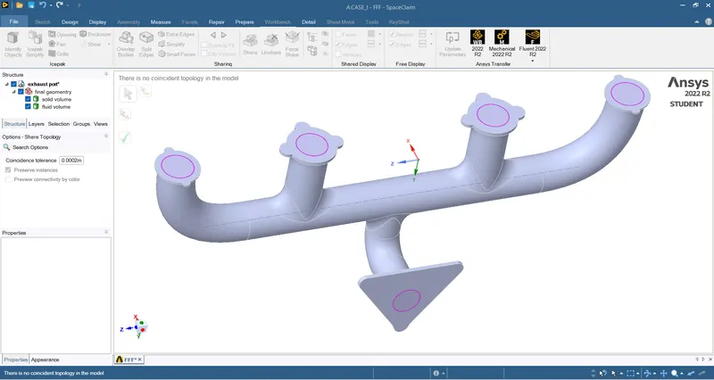
load the model into the space claim and change the unit meter.
if you see extra edges remove them first.
using extract volume select input and output edges, then execute comments.
assign names solid volume and fluid volume as two areas.
assign the final geometry name to move it inside the folder and delete the empty folder.
enable the share function in the main folder and use the shared topology to share all faces.

MESHING SETUP:

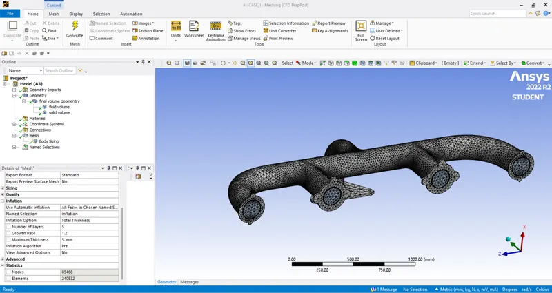
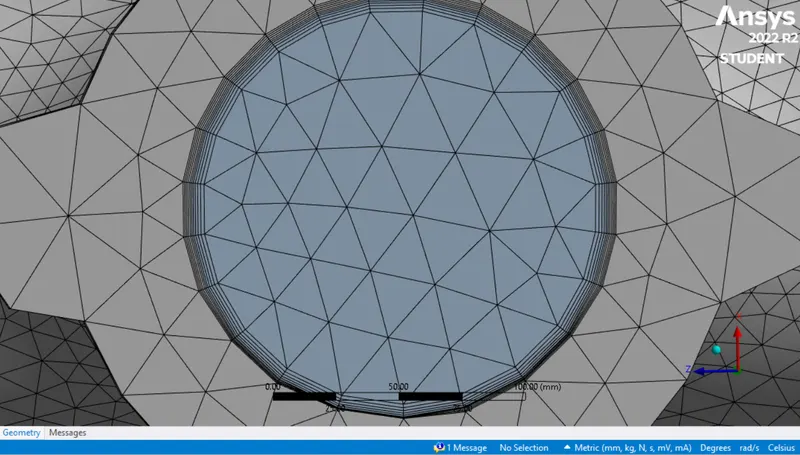
using the name selection tool assigns the name input, output, outer wall convection, and inflation.
using the mesh tool below-mentioned value fill it and get the value of the node and elements.
then close the meshing.

SOLUTION SETUP:

luent setup:

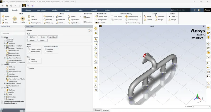
After updating the mesh open fluent setup, select a pressure-based solver using the steady-state time simulation and absolute velocity formulation under the general settings.
Under physics choose the energy option since we are dealing with temperature properties.
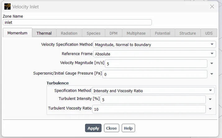
Input the Boundary values at the inlet, 5 m/s as inlet velocity at 700k temperature. Set the outer wall convection boundary to convection type and input a constant value for heat transfer coefficient as 20
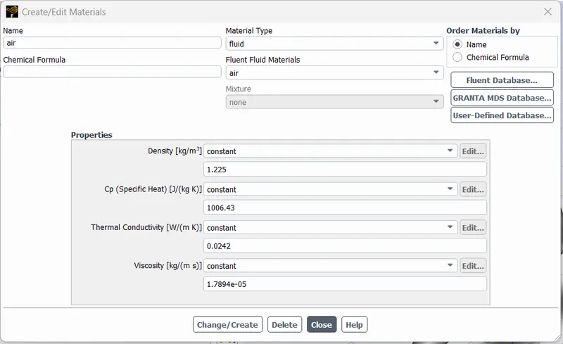
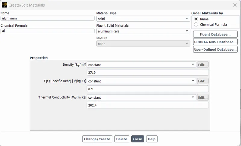
Under materials, properties choose air as the fluid material and aluminum as the solid material
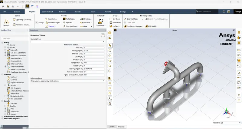
Enter the reference values as per the geometry and inlet boundary conditions accordingly.
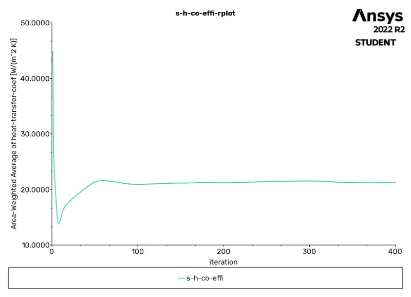
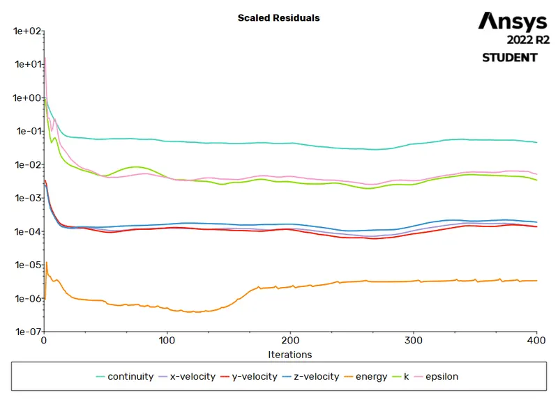
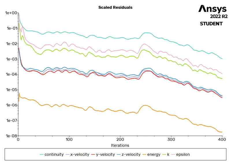
Initialize by using the hybrid initialization, and the simulations for 400 iterations as it is optimum to achieve a converged solution.

Case 1: Baseline simulation

element size =150mm

sizing element size=50mm

no. of elements=240832

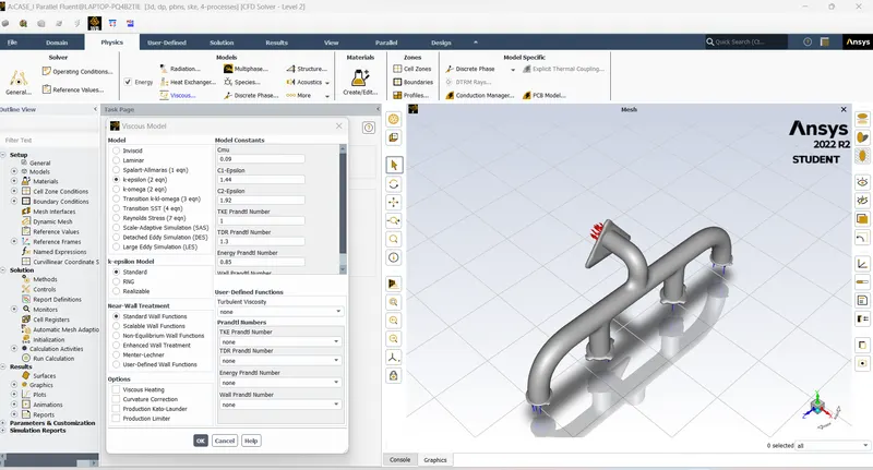
viscous model=k-epsilon

inlet velocity =5m/s

inlet temperature=700k

HT co-efficient=20W/m^2-k

surface heat transfer coefficient :

residuals:

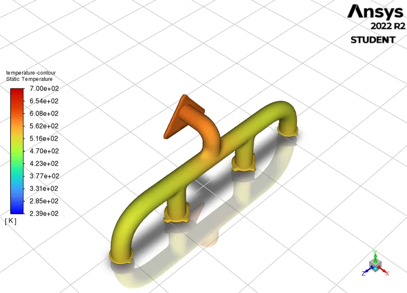
Temperature contour:

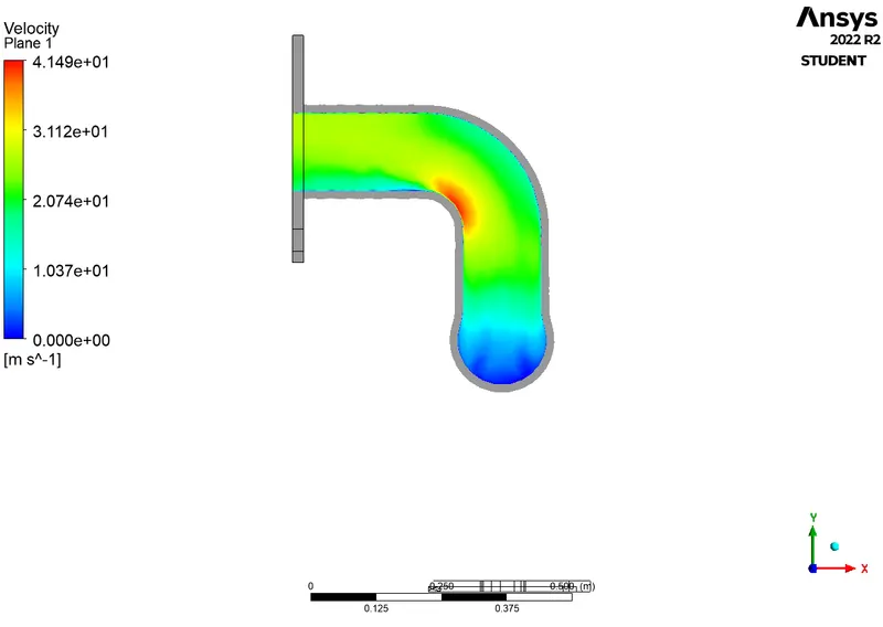
VELOCITY PLOT:

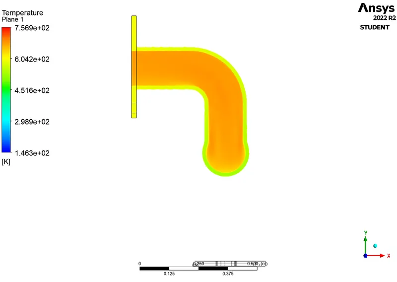
TEMPERATURE PLOT:

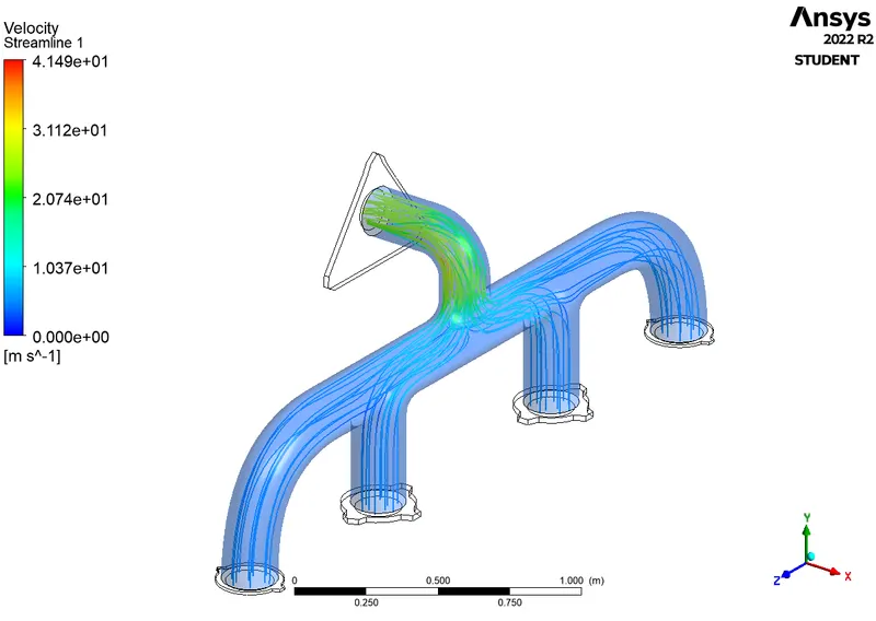
VELOCITY STREAMLINE PLOT:

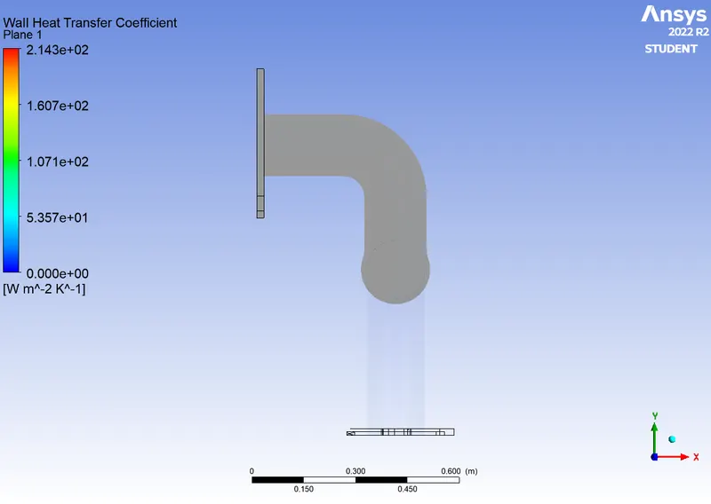
WALL HEAT TRANSFER CO-EFFI:

-------------------------------------------------------------------------------------------------------------------------------

Case 2 :

element size =100mm

sizing element size=20mm

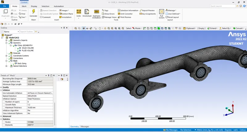
no. of elements=338717

viscous model=k-epsilon

inlet velocity =5m/s

inlet temperature=700k

HT co-efficient=20W/m^2-k

MESHING CONDITION:

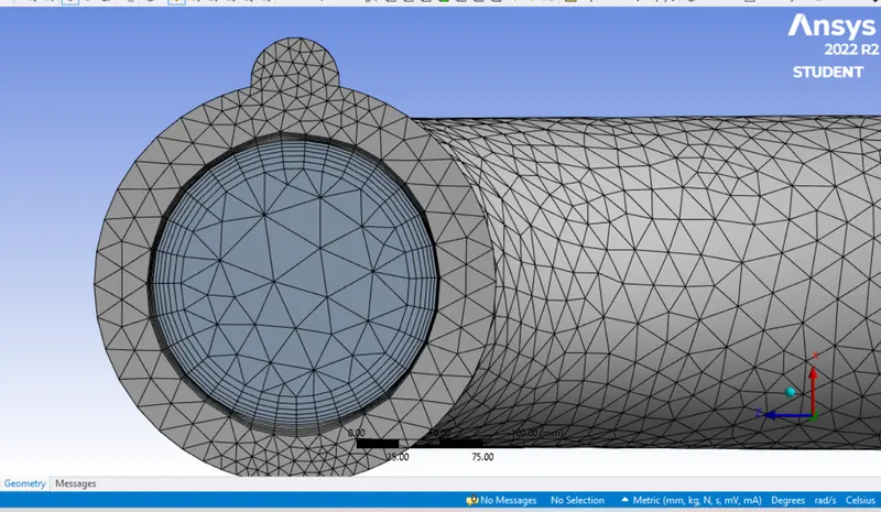
INFLATION :

RESIDUALS:

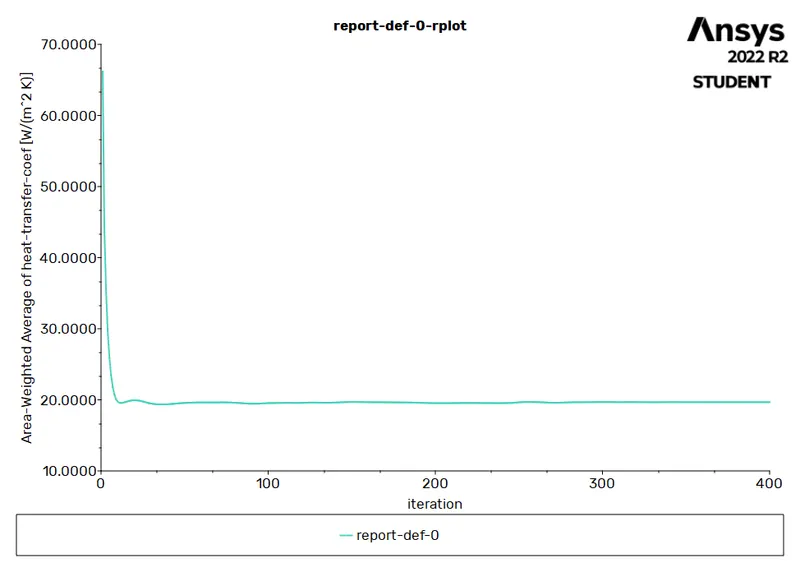
SURFACE HEAT TRANSFER CO EFFICIENT:

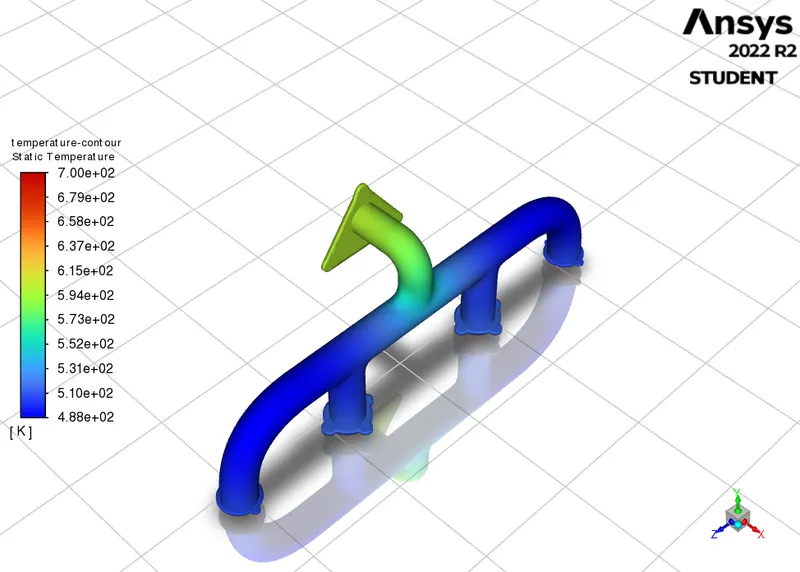
TEMPERATURE CONTOUR:

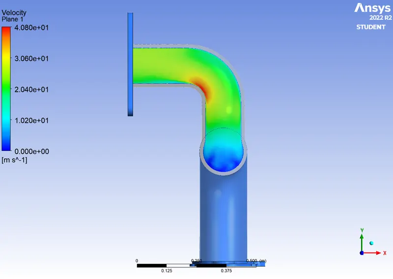
VELOCITY PLOT:

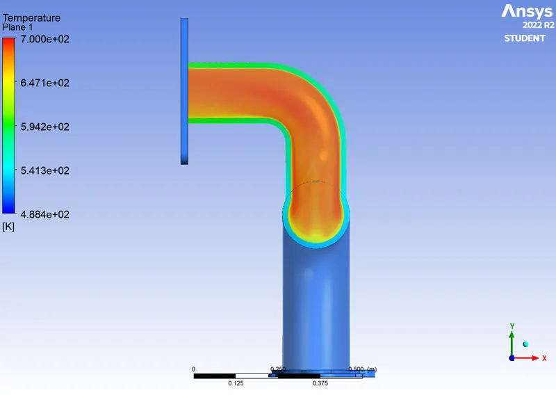
TEMPERATURE PLOT:

VELOCITY STREAMLINE PLOT:

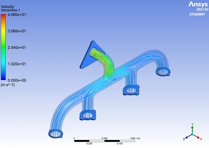
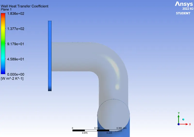
WALL HEAT TRANSFER CO EFFICIENT:

------------------------------------------------------------------------------------------------------------------------------------

Case 3:

element size =100mm

sizing element size=20mm

no. of elements=366372

viscous model=k-omega

inlet velocity =5m/s

inlet temperature=700k

HT co-efficient=20W/m^2-k

MESHING CONDITION:

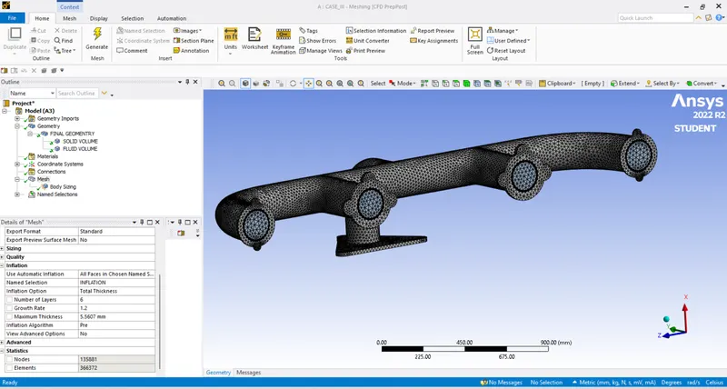
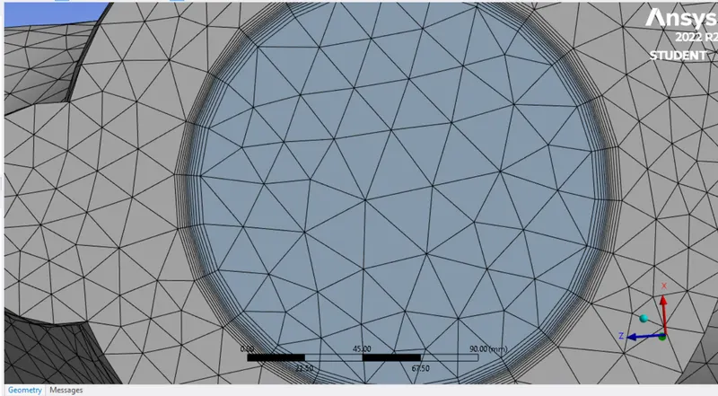
INFLATION:

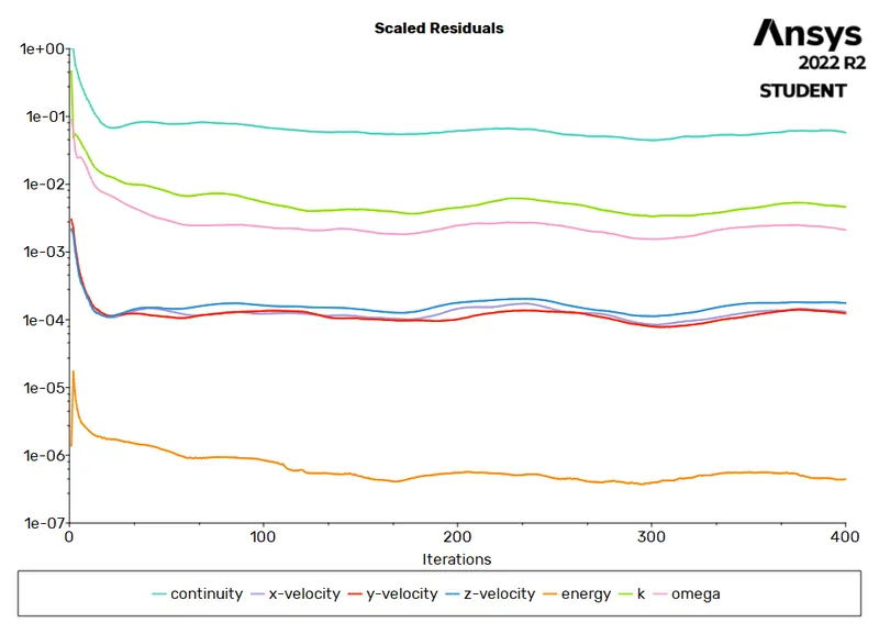
RESIDUALS:

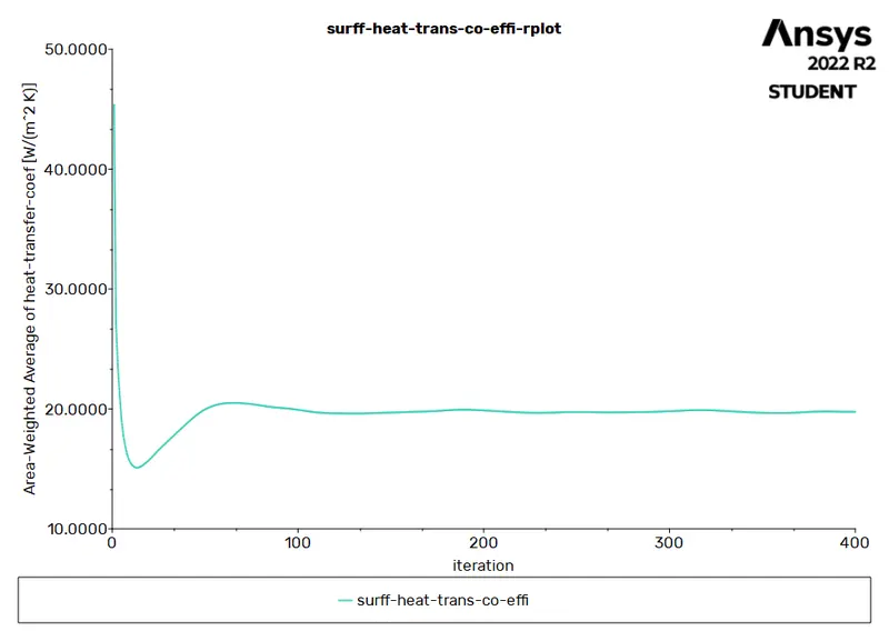
SURFACE HEAT TRANSFER CO-EFFI:

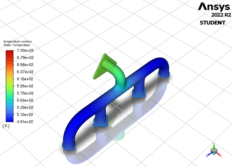
TEMPERATURE CONTOUR:

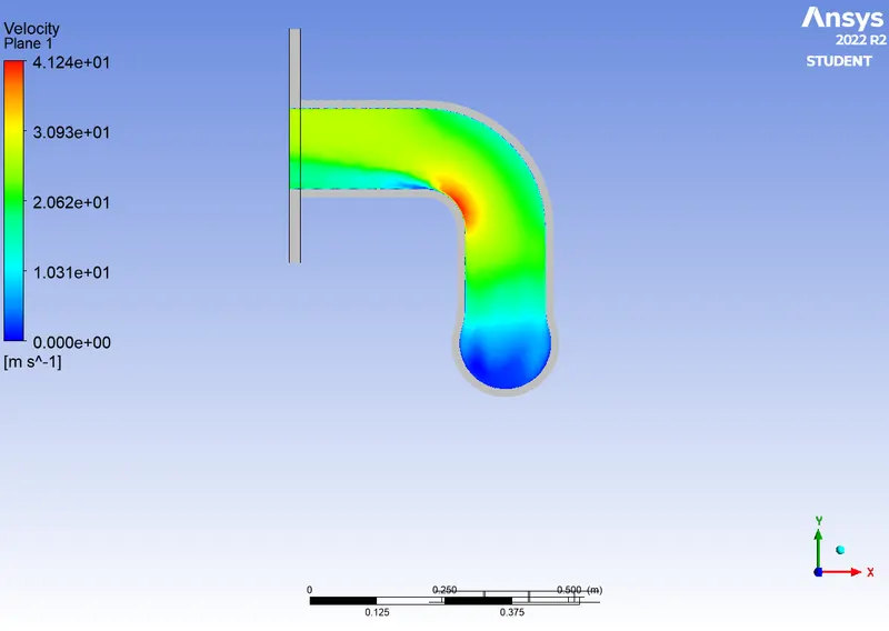
VELOCITY PLOT:

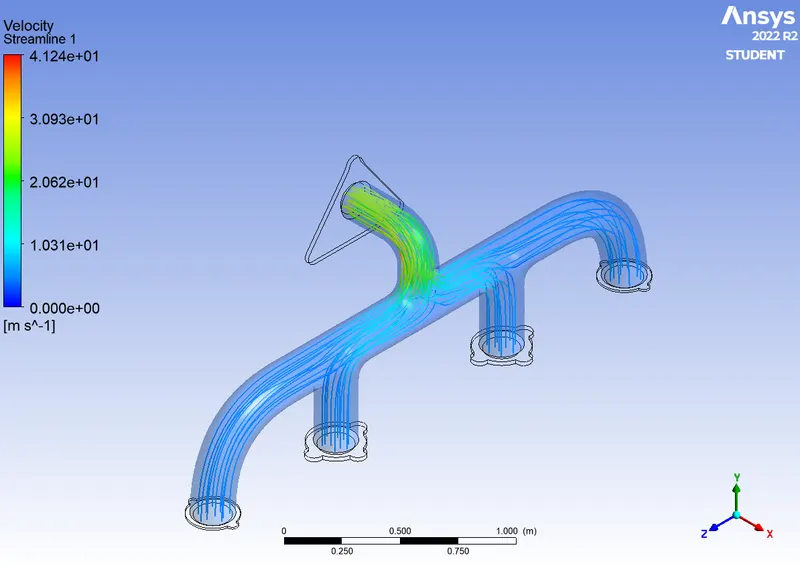
VELOCITY STREAMLINE PLOT:

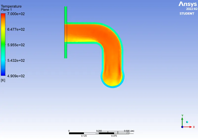
TEMPERATURE PLOT:

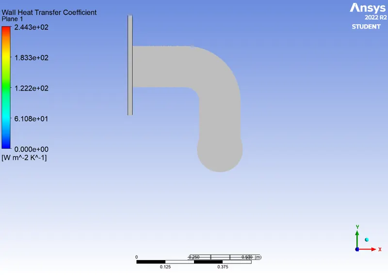
WALL HEAT TRANSFER CO EFFICIENT:

conclusion:

cases	viscous model	no. of elements	surface HT coefficient in(W/m^2-K)	wall HT coefficient in(W/m^2-K)
1	k-epsilon	240832	21.511	214.3
2	k-epsilon(refined)	338717	19.68	183.6
3	k-omega	366372	19.63	244.3

By comparing 3 cases using the k omega model we can get more accurate because we are dealing with temperature

Wall heat co-efficient is more in the k-omega model as compared to k epsilon

There is no change in the temperature for all cases.

Y plus should be calculated depending upon the solvers.

How would you verify if the HTC predictions from the simulations are right? On what factors does the accuracy of the prediction depend on

According to Bernoulli's mass conservation principle mass is conserved in our model which is clearly explained below.

Let us assume the flow rate from each inlet as Q1, Q2, Q3, Q4 respectively, and Q5 be the flow rate(outflow) from the exhaust manifold.

As mass is neither created nor destroyed, mass flow rates are also balanced as below

Q1+Q2+Q3+Q4=Q5Q1+Q2+Q3+Q4=Q5 -------(1)

we have Q=ρ.A.VQ=ρ.A.V -------(2)

now the equation 1 becomes

A1.V1+A2.V2+A3.V3+A4.V4==A5.V5

as it is an incompressible flow to compensate for the mass flow, velocity is increased, and the overall mass flow rate is conserved.

As velocities are high, the Reynolds number at the outlet manifold will be high.

Nu=f(Re, pr) for forced convection applications,

Nu=hD/k

from the above equations

Nu∝Re,

Nu∝h,

hence, Re∝h

From our simulations, we have observed velocities are high at bend section of outlet manifold hence higher Reynolds number which has high Heat transfer coefficients.

Therefore predictions from our simulations can be considered correct.

Factors influence accuracy of prediction:

Mesh quality greatly impacts the accuracy of predicted value from our simulations which can be observed from the above contours and maximum values of related parameters like velocity and heat transfer coefficient.
Appropriate y+ value helps in calculating total layer thickness from the wall for the better capturing of effects near walls, which is HTC in our case.
An appropriate turbulence model has to be used in accordance with the y+ value which is very important
Appropriate solvers are one of the most important factors which lead all the calculations in solving the equations
Inflation layers and boundary conditions

Week 4 - CHT Analysis on Exhaust port

How is Heat Transferred: