Week 4.1 - Genetic Algorithm

AIM:

• Write a code in MATLAB to optimise the stalagmite function and find the global maxima of the function.
• Clearly expalin the concept of genetic algorithm in your own words and also explain the syntax for ga in MATLAB in your report.
• Make sure that your code gives the same output, even if it is made to run several times.
• Plot graphs for all 3 studies and for F maximum vs no. of iterations. Title and axes labels are a must, legends could be shown if necessary.

GENECTIC ALGORITHM:

Genetic algorithm is a search based optimization technique based on the principles of genetics and natural selection. It is frequently used to find optimal or near-optimal solutions. It is frequently used to solve optimization problems, in research, and in machine learning.

WORKING PRICIPLE OF GA:

The algorithm begins by creating a random initial population. The algorithm then creates a sequence of new populations. At each step, the algorithm uses the individuals in the current generation to create the next population.

Scores each member of the current population by computing its fitness value. These values are called the raw fitness scores. Scales the raw fitness scores to convert them into a more usable range of values. These scaled values are called expectation values.

Selects members, called parents, based on their expectation. Some of the individuals in the current population that have lower fitness are chosen as elite. These elite individuals are passed to the next population.

Produces children from the parents. Children are produced either by making random changes to a single parent—mutation—or by combining the vector entries of a pair of parents—crossover. Replaces the current population with the children to form the next generation.

Genetic Algorithm optimization starts with population initialization. Population is the number of sample data points taken to perform the genetic algorithm operation.

GA USEAGE:

Genetic Algorithms are used in optimization problems of various kinds, but they are frequently used in other application areas as well. The areas in which genetic algorithms are frequently used are listed below.

• OPTIMIZATION
• ECONOMICS
• NATURAL NETWORKS
• IMAGE PROCEESSING

Process of natural selection-

The process of natural selection starts with the selection of fittest individuals from a population. They produce offspring which inherit the characteristics of the parents and will be added to the next generation. If parents have better fitness, their offspring will be better than parents and have a better chance at surviving. This process keeps on iterating and at the end, a generation with the fittest individuals will be found. This notion can be applied for a search problem. We consider a set of solutions for a problem and select the set of best ones out of them. Five phases are considered in a genetic algorithm.

1. Initial population

2. Fitness function

3. Selection

4. Crossover

5. Mutation

1.Initial population -The process begins with a set of individuals which is called a Population. Each individual is a solution to the problem you want to solve. An individual is characterized by a set of parameters (variables) known as Genes. Genes are joined into a string to form a Chromosome (solution). In a genetic algorithm, the set of genes of an individual is represented using a string, in terms of an alphabet. Usually, binary values ​​are used (string of 1s and Os). We say that we encode the genes in a chromosome.

2.Fitness fuction-

Fitness Function (also known as the Evaluation Function) evaluates how close a given solution is to the optimum solution of the desired problem. It determines how fit a solution is.

• why we use fitness functions-

In genetic algorithms, each solution is generally represented as a string of binary numbers, known as a chromosome. We have to test these solutions and come up with the best set of solutions to solve a given problem. Each solution, therefore, needs to be awarded a fitness score, to indicate how close it came to meeting the overall specification of the desired solution. This score is generated by applying the fitness function to the test, or results obtained from the tested solution.

3.Selection-

The selectionj is based on the fitness score.The idea of ​​selection phase is to select the fittest individuals and let them pass their genes to the next generation. Two pairs of individuals (parents) are selected based on their fitness scores. Individuals with high fitness have more chance to be selected for reproduction.

4.Crossover-

Crossover is the most significant phase in a genetic algorithm. For each pair of parents to be mated, a crossover point is chosen at random from within the genes. Offspring are created by exchanging the genes of parents among themselves until the crossover point is reached.

5. Mutation-

In certain new offspring formed, some of their genes can be subjected to a mutation with a low random probability. This implies that some of the bits in the bit string can be flipped. Mutation occurs to maintain diversity within the population and prevent premature convergence . termination The algorithm terminates if the population has converged (does not produce offspring which are significantly different from the previous generation).

Then it is said that the genetic algorithm has provided a set of solutions to our problem. The population has a fixed size. As new generations are formed, individuals with least fitness die, providing space for new offspring. The sequence of phases is repeated to produce individuals in each new generation which are better than the previous generation. Ga as function of matlab

DEFINING THE STALAGMITE FUNCTION CODE:

stalagmite =f1.f2.f3.f4

Here,

`f1=[sin(5.1+pix+0.5)]^6`

`f2=[sin(5.1+piy+0.5)]^6`

`f3=exp[-4log(2){(x-0.0667)^2/0.64}]`

`f4=exp[-4log(2){(y-0.0667)^2/0.64}]`

STALAGMITE FUNCTION:

PROGRAM TO MATLAB:

clear all

close all

clc

% Defining search space

x = linspace(0,0.6,150);

y = linspace(0,0.6,150);

% creating 2D grid

[X,Y] = meshgrid(x,y)

for i = 1:length(X)

for j = 1:length(Y)

input_vector(1)=X(i,j);

input_vector(2)=Y(i,j);

F(i,j)=stalagmite_f(input_vector);

end

end

figure(1)

surfc(X,Y,-F)

xlabel('x-value')

ylabel('y-value')

zlabel('F-value')

shading interp

title('Global maxima')

legend('stalagmite','Global maxima')

% study_1:statistical Behaviour

iteration = 50;

tic

for i = 1:iteration

[input,Fopt(i)]=ga(@stalagmite_f,2);

xopt(i) = input(1);

yopt(i) = input(2);

end

study1_time = toc;

figure(2)

subplot(2,1,1)

surfc(X,Y,-F)

xlabel('x-value')

ylabel('y-values')

shading interp

hold on

plot3(xopt,yopt,-Fopt,'Marker','o','MarkerSize',5,'MarkerFaceColor','r')

title('case1:unbounded input')

subplot(2,1,2)

plot(-Fopt)

xlabel('Iteration')

ylabel('function maximum value')

legend('stalagmite')

% study_2: statistical behavior with upper and lower bounds

tic

for i = 1:iteration

[input2,Fopt(i)]=ga(@stalagmite_f,2,[],[],[],[],[0;0],[0.4;0.4]);

xopt(i) = input2(1);

yopt(i) = input2(2);

end

study2_time=toc;

figure(3)

subplot(2,1,1)

surfc(X,Y,-F)

xlabel('x-value')

ylabel('y-value')

shading interp

hold on

plot3(xopt,yopt,-Fopt,'Marker','o','MarkerSize',5,'MarkerFaceColor','r')

title('case 2:Bounded inputs')

subplot(2,1,2)

plot(-Fopt)

xlabel('Iteration')

ylabel('Function maximum value')

legend('stalagmite')

% study_3: statistical behaviour with input and increased population size

options = optimoptions('ga');

options = optimoptions(options,'PopulationSize',100);

tic

for i = 1:iteration

[input3,Fopt(i)]=ga(@stalagmite_f,2,[],[],[],[],[0;0],[0.4;0.4],[],[],options);

xopt(i) = input3(1);

yopt(i) = input3(2);

end

study3_time=tic;

figure(4)

subplot(2,1,1)

surfc(X,Y,-F)

shading interp

xlabel('x-value')

ylabel('y-value')

hold on

plot3(xopt,yopt,-Fopt,'Marker','o','MarkerSize',5,'MarkerFaceColor','r')

title('case 3: bounded inputs with increased population size')

subplot(2,1,2)

plot(-Fopt)

xlabel('Iteration')

ylabel('Function maximum value')

legend('Iteration')

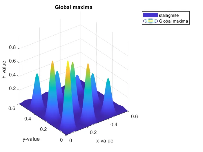
EXPLANATION FOR CODE:

• using clear all,close all,clc is clear to workspace,commond window,figure window.
• using linspace commond to take 150 values from 0 to 0.6.
• meshgrid using to take 3d plot.
• using for loop for i& j to gives inputs values.
• using stalagmite function to take initial condition.
• figure(1) for to get first figure window.
• using surface commond to define surface by z coordintes of points above a rectangular grid in x-y plane.
• using xlabel and ylabel and zlabel to gives the x and y and f values.
• shading interp using to various the color i each line segment and face.
• title commond to give title.
• using legend commond to give title.

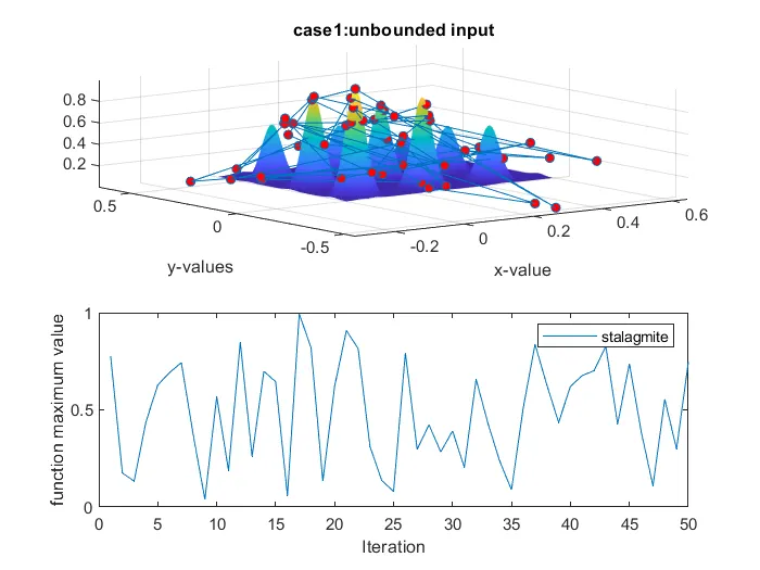
study_1:statistical Behaviour code explanation:

• using tic and toc commond to report the total time required for element by element matrix multiplication purpose.
• using subplot commond divides the current figure into rectangular panes the are numbered row wise.
• shading interp using to various the color i each line segment and face.
• using plot3 to get plot the values of xopt,yopt and -Fopt.
• title commond to give title.
• using subplot commond divides the current figure into rectangular panes the are numbered row wise
• using xlabel and ylabel and zlabel to gives the x and y values.
• using legend commond to give title.

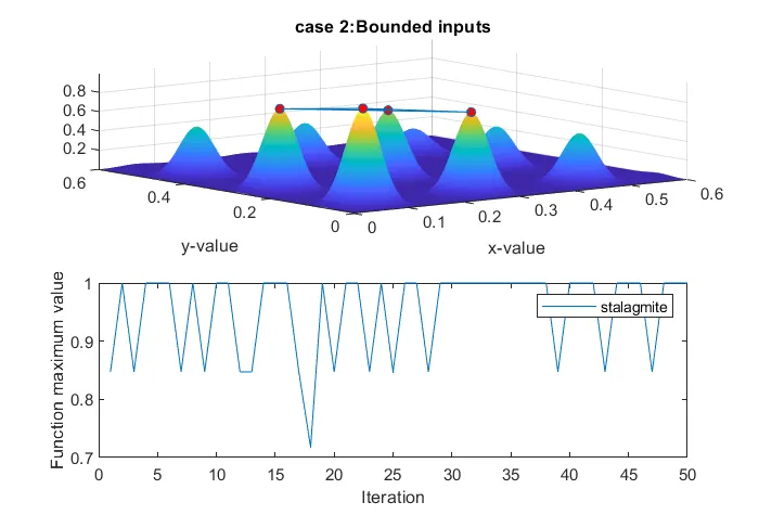
• using tic and toc commond to report the total time required for element by element matrix multiplication purpose.
• using subplot commond divides the current figure into rectangular panes the are numbered row wise.
• shading interp using to various the color i each line segment and face.
• using plot3 to get plot the values of xopt,yopt and -Fopt.
• title commond to give title.
• using subplot commond divides the current figure into rectangular panes the are numbered row wise
• using xlabel and ylabel and zlabel to gives the x and y values.
• using legend commond to give title.

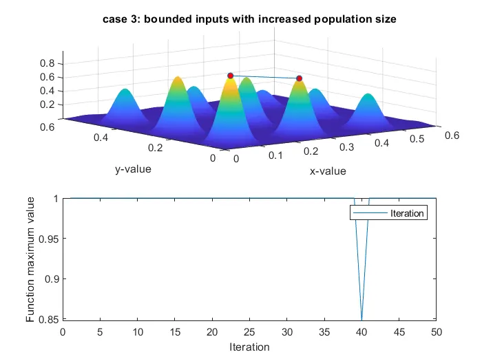
study_3: statistical behaviour with input and increased population size code explanation:

• using options to give 'ga'.
• using options to optimoptions to give 100 increased populationsize.
• using tic and toc commond to report the total time required for element by element matrix multiplication purpose.
• using subplot commond divides the current figure into rectangular panes the are numbered row wise.
• shading interp using to various the color i each line segment and face.
• using plot3 to get plot the values of xopt,yopt and -Fopt.
• title commond to give title.
• using subplot commond divides the current figure into rectangular panes the are numbered row wise
• using xlabel and ylabel and zlabel to gives the x and y values.
• using legend commond to give title.

ERROR USING WHILE PROGRAMMING:

Basic typing mistake error.

CONCLUTION:

Thus we have optimized stalagmite function and found the global maxima for the function.

WHILE PROGRAMMING VIDEO LINK:

https://drive.google.com/file/d/171hQo1WSrWZ2PveP5nQtUctNx_adqBh2/view?usp=sharing