Project 2 - Rankine cycle Simulator

AIM:

To Programme a Rankine Cycle Simulator using MATLAB.

OBJECTIVES:

• Create a Rankine Cycle Simulator using OCTAVE/MATLAB.
• Your code should calculate the state points of the Rankine Cycle (any type of your choice) based on user inputs.
• Then, plot the corresponding T-s and h-s plots for the given set of inputs. Title and axes labels are a must, while legends could be used if necessary.

RANKINE CYLCLE THEORY:

The Rankine cycle is the fundamental operating cycle of all power plants where an operating fluid is continuously evaporated and condensed. The selection of operating fluid depends mainly on the available temperature range.

• Process 1–2: The working fluid is pumped from low to high pressure. As the fluid is a liquid at this stage, the pump requires little input energy. Process 1-2 is isentropic compression.
• Process 2–3: The high-pressure liquid enters a boiler, where it is heated at constant pressure by an external heat source to become a dry saturated vapour. The input energy required can be easily calculated graphically, using an enthalpy–entropy chart (h–s chart, or Mollier diagram), or numerically, using steam tables or software. Process 2-3 is constant pressure heat addition in boiler.
• Process 3–4: The dry saturated vapour expands through a turbine, generating power. This decreases the temperature and pressure of the vapour, and some condensation may occur. The output in this process can be easily calculated using the chart or tables noted above. Process 3-4 is isentropic expansion.
• Process 4–1: The wet vapour then enters a condenser, where it is condensed at a constant pressure to become a saturated liquid. Process 4-1 is constant pressure heat rejection in condenser.

1 – 2 : Isentropic Compression in a Pump.

2 – 3 : Constant Pressure Heat Addition in a Boiler.

3 – 4 : Isentropic Expansion in a Turbine.

4 – 1 : Constant Pressure Heat Rejection in Condenser.

MATHEMATICAL EQUATIONs:

• Net Work done (W_Net) = W_Turbine – W_pump ;
• Thermal Efficiency (η) = W_Net / Q_in ;
• Work Ratio (WR) = W_Net / W_Turbine ;
• Back Work Ratio (BWR) = W_Pump / W_Turbine ;
• WR + BWR = 1 ;
• Heat Rate (HR) = 1/ η ;
• Steam Rate (SSC) = 1 / W_Net ;

CODE FOR RANKINE CYCLE SIMULATOR:

clear all
close all
clc

% script for different state points
% 1 = turbine inlet or boiler outlet.
% 2 = condenser inlet or turbine outlet
% 3 = pump inlet or condenser outlet
% 4 = boiler inlet or pump outlet

% input parameters
% p1 = turbine inlet pressure in bar
% T1 = temperature at turbine inlet (degree C)
% p2 = turbine outlet pressure in bar

fprintf('process (1-2)-Isentropic Expansion in the Turbine \n');
fprintf('process (2-1)-Isentropic Heat Rejection by the condenser \n');
fprintf('process (3-4)-Isentropic compression in the pump \n');
fprintf('process (4-1)-Isentropic Heat Addition in the boiler \n');

% Input state Variable at point 1
p1 = input('Enter the pressure at the Turbine inlet (in bar) :->\n');
T1 = input('Enter the Temperature at the Turbine inlet (in Degree C) :->\n');
p2 = input('Enter the pressure at the Turbine outlet (in bar) :->\n');

% calculating state variables at all points from given data file
% getting cp & cv from 'XSteam'
% for vapour
high_cpV = XSteam('CpV_p',p1);
low_cpV  = XSteam('CpV_p',p2);
high_cvV = XSteam('CvV_p',p1);
low_cvV = XSteam('CvV_p',p2);

% for liquid
high_cpL = XSteam('CpL_p',p1);
low_cpL  = XSteam('CpL_p',p2);
high_cvL = XSteam('CvL_p',p1);
low_cvL = XSteam('CvL_p',p2);

% getting important parameters from 'XSteam' data file.
% For high pressure
T1s = XSteam('Tsat_p',p1);
s1g = XSteam('sV_p',p1);
s1f = XSteam('sL_p',p1);
s1fg = s1g-s1f;
h1f = XSteam('hL_p',p1);
h1g = XSteam('hV_p',p1);
h1fg=h1g-h1f;

%For low pressure
T2s = XSteam('Tsat_p',p2);
s2g = XSteam('sV_p',p2);
s2f = XSteam('sL_p',p2);
s2fg = s2g-s2f;
h2f = XSteam('hL_p',p2);
h2g = XSteam('hV_p',p2);
h2fg=h2g-h2f;

% state variable at point 1
fprintf('At state 1 :-------->\n');
fprintf('p1 is : %f bar \n',p1);
fprintf('T1 is : %f Degree C \n',T1);
h1 = XSteam('h_pT',p1,T1);
fprintf('h1 is : %f kJ/kg \n',h1);
s1 = XSteam('s_pT',p1,T1);
fprintf('s1 is : %f kJ/kgk \n',s1);

% state variables at point 2
fprintf('At state 2 :------> \n');
fprintf('p2 is : %f bar \n',p2);
% entropy remains the same through turbine (ideal)
s2 =s1;
fprintf('s2 is : %f kJ/kgk \n',s2);
% calulate value of 'x' drayness fraction
if (s2 <= s2g)
    x2 = (s2-s2g)/(s2fg);
else
    x2=1;
end
fprintf('x2 is : %f \n',x2)
% calculate the value of 'T2'
if (x2<1)
    T2 = T2s;
else
    T2 = (T2s+273.15)*exp((s2-s2g)/low_cpV);
    T2 = T2-273.15;
end 
fprintf('T2 is : %f Degree C \n',T2);
% for calculating value of h2
if (x2<1)
    h2 = h2f+x2*h2fg;
else
    h2 = h2g+low_cpV*(T2-T2s);
end
fprintf('h2 is : %f kJ/kg \n',h2);

% state variables at point 3
fprintf('At state 3 :-------->\n')
p3 = p2;
fprintf('p3 is : %f bar \n',p3)
V3 = XSteam('vL_p',p3);
T3 =T2s;
fprintf('T3 is : %f Degree C \n',T3);
h3=h2f;
fprintf('h3 is : %f kJ/kg \n',h3);
s3 =s2f;
fprintf('s3 is : %f kJ/kgk \n',s3);

% state variables at point 4
fprintf('At state 4 :-------->\n')
p4 =p1;
fprintf('p4 is : %f bar \n',p4);
s4 =s3;
fprintf('s4 is : %f kJ/kgk \n',s4);
T4 = XSteam('T_ps',p4,s4);
fprintf('T4 is : %f Degree C \n',T4);
W_p = V3*(p4-p3)*100;
h4 = W_p+h3;   % work done by pump (W_p)=h4-h3
fprintf('h4 is : %f kJ/kg \n',h4);

% Work done by the turbine
W_T = h1-h2;
fprintf('Work Done by the Turbine is : %f kJ/kg \n',W_T);
fprintf('Work Done by the Pump is : %f kJ/kg \n',W_p);

% Net Work Done
Wnet = W_T-W_p;
fprintf('Net Work Done is : %f kJ/kg \n',Wnet);

% Net Heat Supplied
Qin = h1-h4;
Qout = h2- h3;

% Thermal efficiency
eff_thermal = Wnet/Qin;
fprintf('Thermal Efficiency is : %f \n',eff_thermal);

% Back Work Ratio
b_w_r = (W_p/W_T);
fprintf('Back Work Ratio is : %f \n',b_w_r);

% Work Ratio
w_r = (Wnet/W_T);
fprintf('Work Ratio is %f \n',w_r);

% summation of b_w_r and w_r should be 1
fprintf('Back Work Ratio + Work Ratio is : %f \n',(b_w_r+w_r))

% Heat rate and specific steam cosumption
H_R = (1/eff_thermal);
fprintf('Heat Rate is : %f kJ/kWs \n',H_R)
ssc = (3600/W_T);
fprintf('Specific Steam Consumption is : %f kg/kWh \n',ssc)

% Itearing saturation liquid and vapour line from 0 to T1
temperature = linspace(0,T1,5000);
for i = 1:length(temperature)
    h_L(i) = XSteam('hL_T',temperature(i));
    h_V(i) = XSteam('hV_T',temperature(i));
    s_L(i) = XSteam('sL_T',temperature(i));
    s_V(i) = XSteam('sV_T',temperature(i));
end
 
% plotting saturated curve for T-s Diagram
plot(s_L,temperature,'red','LineStyle','--','LineWidth',1)
hold on
plot(s_V,temperature,'blue','LineStyle','--','LineWidth',1)

% plot T-S diagram
figure(1)
hold on
plot([s1 s2],[T1 T2],'Color','yellow','LineWidth',3)
plot([s2 s2g],[T2 T2s],'Color','green','LineWidth',3)
plot([s2g s3],[T2s T3],'Color','green','LineWidth',3)
plot([s3 s4],[T3 T4],'Color','yellow','LineWidth',3)
plot([s4 s1f],[T4 T1s],'Color','yellow','LineWidth',3)
plot([s1f s1g],[T1s T1s],'Color','green','LineWidth',3)
plot([s1g s1],[T1s T1],'Color','green','LineWidth',3)
legend('saturated liquid curve','saturated vapour curve')
text(s1,T1,'1','FontSize',15)
text(s2,T2,'2','FontSize',15)
text(s2g,T2s,'2s','FontSize',15)
text(s3,T3,'3','FontSize',15)
text(s4,T4,'4','FontSize',15)
text(s1f,T1s,'4s','FontSize',15)
text(s1g,T1s,'1s','FontSize',15)

% making direction
text(s1,(T1+T2)/2,'\vee','Color','yellow')
text((s2g+s2f)/2,T3,'\angle','Color','yellow')
text(s3,(T3+T4)/2,'\wedge','Color','yellow')
text((s1f+s1g)/2,T1s,'\angle','color','yellow')
axis([0 10 0 500])
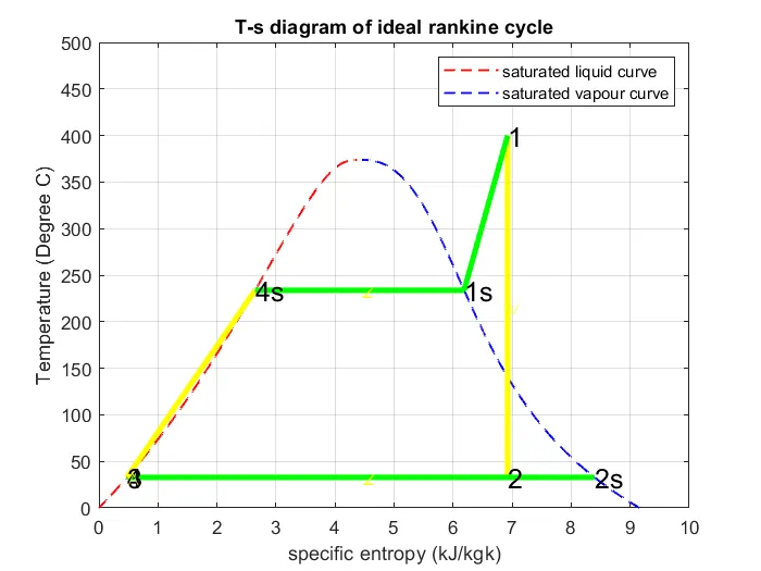
title('T-s diagram of ideal rankine cycle')
xlabel('specific entropy (kJ/kgk)')
ylabel('Temperature (Degree C)')
grid on

% plot h-s diagram
figure(2)
plot(s_L,h_L,'Color','black','LineStyle','--','LineWidth',1)
hold on
plot(s_V,h_V,'Color','red','LineStyle','--','LineWidth',1)
plot([s1 s2],[h1 h2],'Color','yellow','LineWidth',3)
plot([s2 s3],[h2 h3],'Color','green','LineWidth',3)
plot([s3 s4],[h3 h4],'Color','yellow','LineWidth',3)
plot([s4 s1],[h4 h1],'Color','green','LineWidth',3)
text(s1,h1,'1','FontSize',15)
text(s2,h2,'2','FontSize',15)
text(s3,h3,'3','FontSize',15)
text(s4,h4,'4','FontSize',15)
title('h-s Diagram of Ideal Rankine cycle')
xlabel('Specific Entropy (kJ/kgk)')
ylabel('Specific Enthalpy (kJ/kg)')
legend('saturated liquid curve','saturated vapour curve')
grid on

CODE EXPLANATION:

• Clear all: for clears all the data stored in the workspace previously.
• Close all: for closes all the previous figures and plots.
• clc: for clears the command window.
• To simulate and find out different state variables, all the processes parameters are to be described such as all four processes occurring and inputs parameters.
• From the standard ‘X-steam’ data is used to extract steam and water properties of Enthalpy, Entropy at specific pressure and temperatures for saturated liquid and vapour conditions etc.
• The program requires the input of pressure (in bar) at turbine inlet, Temperature at turbine inlet (degree C) and pressure at the turbine outlet(in bar

INPUT IS

Enter the Pressure at the Turbine Inlet (in bar): -> 30

Enter the Temperature at the Turbine Inlet (in Degree C ): -> 400

Enter the Pressure at the Turbine Outlet (in bar): -> 0.05

• With the help of these inlets & from ‘Xsteam’ data, the program calculates all the state points of the Rankine cycle.

The ‘Xsteam’ data works as, h1=XSteam(h_pT,p1,T1) it returns the Enthalpy, Entropy at specific pressure and temperatures in bar and Degree C respectively.

• As we extract the data, we use thermodynamics relations to further find state points and extract their data from XSteam data file which are mentioned after studying the Rankine cycle.
• ‘sf’ and ‘sg’ & ‘hf’ and ‘hg’, where f and g stands for saturated liquid and vapour respectively are calculated after studying the plots of Rankine cycles and extracting data from Xsteam file.
• The net work done, work done by turbine, work by pump, thermal efficiency, back work ratio, work ratio, heat rate, heat in, heat out, specific steam consumption are calculated using standard thermodynamics relations and mentioning them in program using those relations.
• To plot the property diagram of water, i.e., saturation liquid and vapour line, an array is created using ‘linspace’ command from 0 to value of T1 with 5000 evenly spaced points in between them and suitable state variables are iterated using ‘for’ loop.
• T, s and h are extracted at vapour and liquid line for plotting purpose, after 4^th point for the variation observed in the plot.
• Saturation curve is plotted in ‘----’ for saturated liquid & gas in T-s and h-s graph’s, also with all the required points are plotted and marked using ‘text’ command
• The plots changes as the user input changes for the above mentioned inputs.
• Results are displayed in the command window by using ‘fprintf’ command.

1. Line6-9mentions all 4 processes using ‘fprintf’ command.
2. Line12-14// create input state variables at point1.(for p1,T1,p2)
3. Line26-119// calculating state variables at all points from given datafile (XSteam),

Get those data form ‘XSteam’ file and calculate those data using standard thermodynamic formulas for finding ‘p,T,h,s’ etc. at all state points (1,2,3,4) & print those final ‘p,T,h,s’ values using ‘fprintf’ command at all points.

4. Line121-175// calculating Net work output, net heat, back work ratio, Thermal efficiency, heat rate & specific steam consumption using formula and print it for getting the output results.
5. Line177-162// for saturation liquid and vapour line, an array is created using ‘linspace’ command from 0 to value of T1 with 5000 evenly spaced points in between them and suitable state variables are iterated using ‘for’ loop.
6. Line164-167// plotting of saturated curve for T-s diagram using ‘plot’ command.
7. Line169-179// for figure1 (T-s diagram) plot all following paths and put ‘color’ and ‘linewidth’ commands after that using ‘legend’ command for mention the saturated liquid and vapour curve.
8. Line180-186// using ‘text’ command for mark those all four state points. & use ‘fontsize’ command for give a suitable size of all those lines.
9. Line189-197// put a proper dimension of the figure using ‘axis’ command, ‘title’ command for giving a title of the graph, label it with specific parameters, ‘grid on’ command is enable.
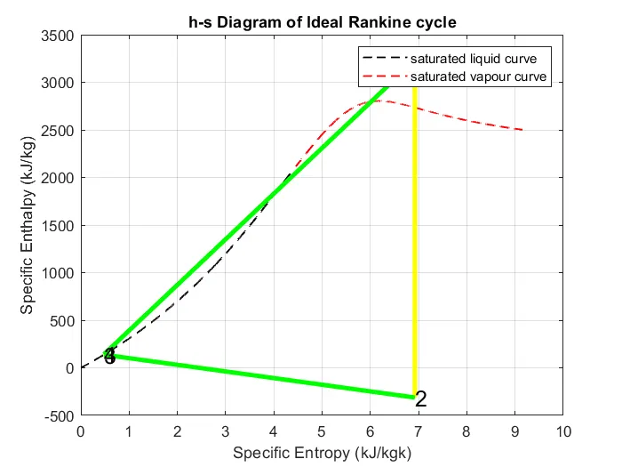
10. Line199-216// at last for figure2 (h-s diagram) do the same process, plot all points, give text for mark state points, then give the title and label it properly with specific parameters for fig2. ‘legend’ also use for mark saturated curve in the diagram & enable the grid.

RESULT:

PLOT FOR T-S DIAGRAM

PLOT FOR H-S DIAGRAM:

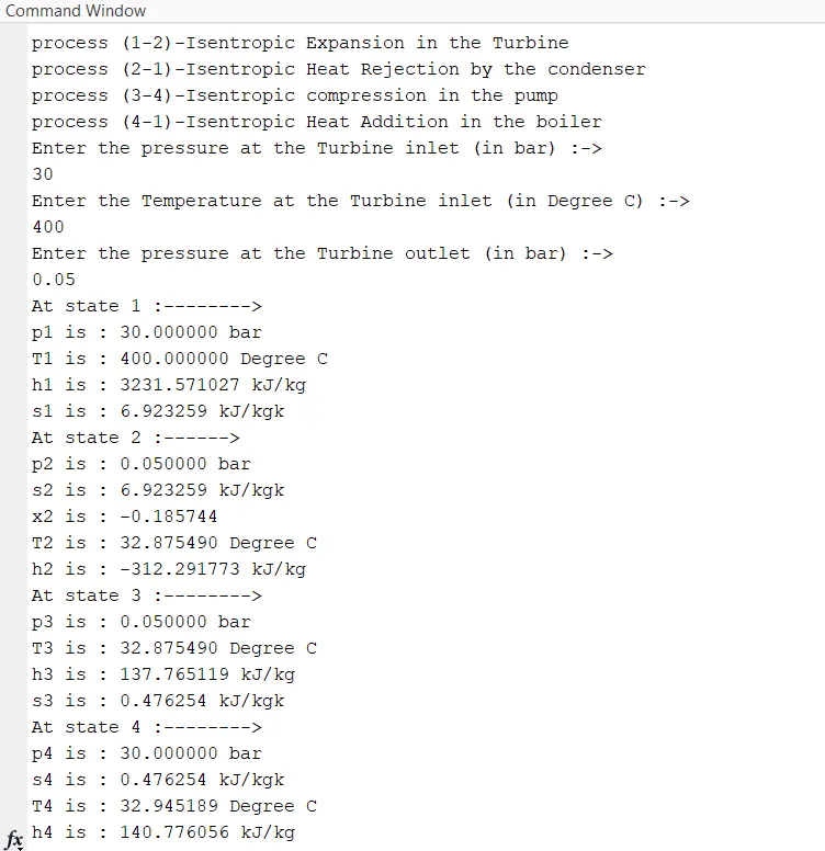
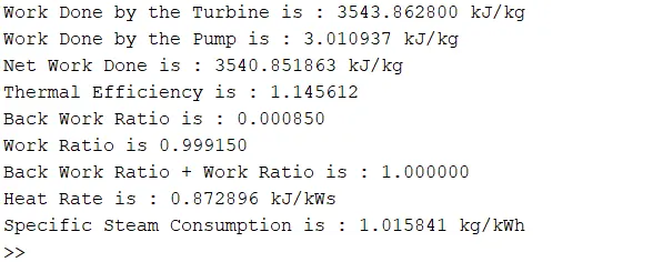
CALCULATING FOLLOWINGS:

Back Work Ratio is : 0.000850

Net Work Done is : 3540.851863 kJ/kg

CONCLUSION:

In this program, reheat and regenerative cycles of Rankine cycle can be simulated.From it we get the values of all state points, & program also generate all it's simulation equations behalf of my primary input values. Also we get T-s & h-s plots of Rankine cycle.

DURING WRITE A CODE VEDIO LINK:

https://drive.google.com/file/d/1Yjpzw9RVdkiZuHkmtIU2v-GoIb4KjYvV/view?usp=sharing