Week 3 - Solving second order ODEs
OBJECTIVE:
write a program that solves the following ODE. This ODE represents the equation of motion of a simple pendulum with damping.
THE SECOND ODER ODE EQUATION IS
Newton second law of rotational systems,the equation of motion of the pendulum may be obtained
`(d^2theta)/dt+gLsintheta=0`
In the case of a damper with damping co-efficient 'b',the equation chage to
`(d^2theta)/dt^2+b/m(d theta)/dt+g/L(sin theta)=0`------------(1)
In order to order ODEconvert 2nd order ODE to 1 st order ODE ,let make some assume,
`theta=theta1`
therefore
`(d theta)/dt=(d theta1)/dt`
Also let,
`(d theta1)/dt=theta2`---------(2)
Therfore
`(d^2 theta)/dt^2=(d theta2)/dt`------(3)
We have a two condition 2&3 ,apply to 1 condition
`ⅆ/(ⅆt) [θ_1/θ_2 ]=[█θ_2@-b/m×(θ_2 )-g/L sin(θ_1 ) ]`
To solve this condition of first order ODE,matlb has function ODE45
INPUT PARAMETERS:
L=1 metre, % L = length of the pendulum in m,
m=1 kg, % m = mass of the ball in kg,
b=0.05. % b=damping coefficient.
g=9.81 m/s2. % g = gravity in m/s2,
Simulate the motion between 0-20 sec, for angular displacement=0,angular velocity=3 rad/sec at time t=0.
FUNCTION TO DEFINE SOLUTION MATRIX THETA:
FUNCTION CODE EXPLANATION:
- Write the function code to use variable name ode_func_result with our input parameters.
- theta (1) value is assigned variable called theta 1.
- theta (2) value is assigned variable called theta 2.
- Apply to (d theta1)/dt=theta2
- Apply to (d theta2)/dt=-(b/m)*theta2-(g/l)*sin(theta1);
- Apply to `ⅆ/(ⅆt) [θ_1/θ_2 ]=[█θ_2@-b/m×(θ_2 )-g/L sin(θ_1 ) ]`using column vector (;)
PROGRAM TO MAKE PLOTTING FOR DISPLACEMENT AND VELOCITY
- clear all,close all,and clc is basically used for worksapce,commond window,and figure window clear to privious data.
- And writting our given parameters values.
- Initial condition is our given values angular displacement and angular veelocity to make theta_0=[0;3] .
- Limit of intergration is our t=0 to t=20 between 200 limits.using linspace commond.
- After that calling the ode function to solve ODE solver.
- when we using the ode45 solver. we need to three term(function to be intergated,time_span,and initial conditions).
- Apply as per our solver terms and after that going to make a plotting.
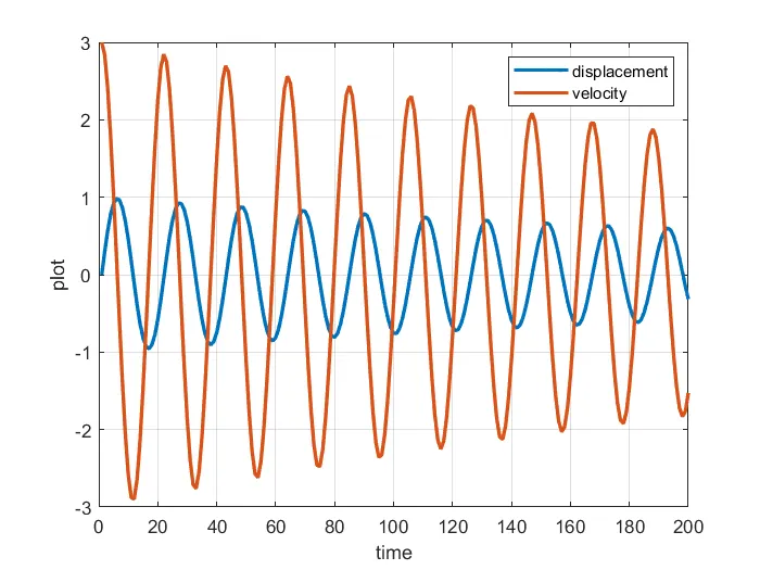
- Using plot commond fill our first row of displacement.
- using hold on commond,because another one is remaining.
- Using plot commond fill our first row of velocity.
- using xlabel and ylabel commond insert our time and plot.
- using grid on
- finally using hold off commond and exicute the program,getting our displacement and velocity figure
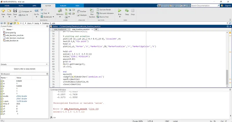
% making animation :
- first write counter commond giving to value 1
- Using for loop respect to time write the condition.
- And write our starting point of pendulum.which mean base.
- write the end point of ball
- Using plot comond write the base point coordination
- And using text commond write the fix point and as size.
- Using hold on commond,because another one is remaining.
- Using plot commond give to end of pendulum.
- Using marker commond give to size ,colour values.
- Using hold off commond.
- Give to axis values for pendulum movement.
- Using pause commond and grid on.
- For make a animation use this term M(ct)=getframe(gcf);
- finall using end commond.
- After that using movie commond.
- using videofile commond give to videowriter as our title and video format.
- Using open commond
- Then write the file in M
- Finally close the video file ,go to RUN the program.
PLOT DISPLACEMENT AND VEVLOCITY:
ANIMATION OF SIMPLE PENDULUM:
CONCLUTION:
Various plot which generate is shown as OUTPUT of program after body of code.
ERROR FACING WHILE PROGRAMMING:
- Basic typing mistakes.
- MATLAB HANGING PROBLEM
Typing erron in axis then corrected.