Week 4 - CHT Analysis on Exhaust port
CONJUGATE HEAT TRANSFER ANALYSIS ON EXHAUST PORT
AIM:
To perform conjugate heat transfer analysis on exhaust port.
OBJECTIVE:
1. To Calculate the wall/surface heat transfer coefficient on the internal solid surface
2. Plot the velocity & temperature contours in appropriate areas.
3. To Discuss the factors involved in the accuracy of the prediction.
INTRODUCTION:
Conjugate heat transfer (CHT) analysis is generally used when there is temperature variation during heating or cooling in the material due to the interaction between solid and fluid phases. It is the combination of heat transfer in solids to heat transfer in fluids. In solids, conduction often dominates whereas in fluids, convection usually dominates. Efficiently combining heat transfer in fluids and solids is the key to designing effective coolers, heaters, or heat exchangers. Forced convection is the most common way to achieve high heat transfer rate. In some applications, the performances are further improved by combining convection with phase change (for example liquid water to vapor phase change).
Examples of Conjugate Heat transfer analysis:
HVAC, Heat Exchanger, Tank, Internal Combustion Engine, Heat Pipe, Turbocharger.
MODELLING APPROACH:
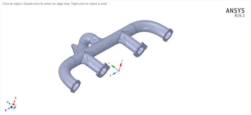
Importing the Geometry in Spaceclaim,
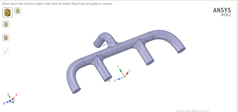
Extract the fluid volume only,
Prepare > Volume Extract > selecct Edges > then Click finish
MESHING
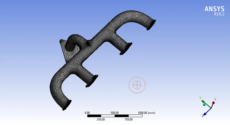
| MESH INPUTS - BASE MESH | |
| Element Size | 150 mm |
| Max Element size | 300 mm |
| Mesh Type | Triangular |
| Nodes | 33743 |
| Elements | 138664 |
| Inflation Layers | - |
| Total Thickness | - |
For Base mesh,
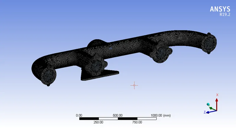
For Refined Mesh,
| MESH INPUTS - REFINED MESH | |
| Element Size | 10 mm |
| Max Element size | 20 mm |
| Mesh Type | Triangular |
| Nodes | 381802 |
| Elements | 1462149 |
| Inflation Option | Total Thickness |
| Inflation Layers | 5 |
| Total Thickness | 5 mm |
SOLVER SETUP
| SOLVER INPUTS | |
| Solver Time | Steady |
| Solver Type | Pressure Based |
| Energy | On |
| Models | K - Omega Standard |
| Material | air |
| Inlet velocity | 5m/s |
| Inlet Temperature | 426.85℃ |
| Thermal Condition | Convection |
| Heat transfer Coefficient | 20 (w/m2k) |
| Iterations | 200 |
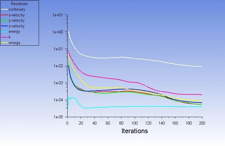
Residual Plot for Base mesh,
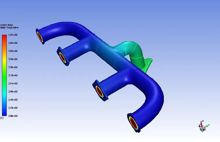
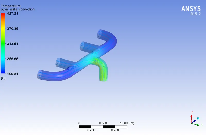
Temperature distribution Plot for base mesh,
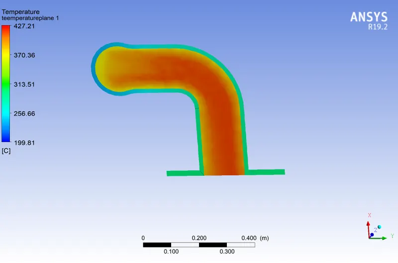
Temerature plot for base mesh,
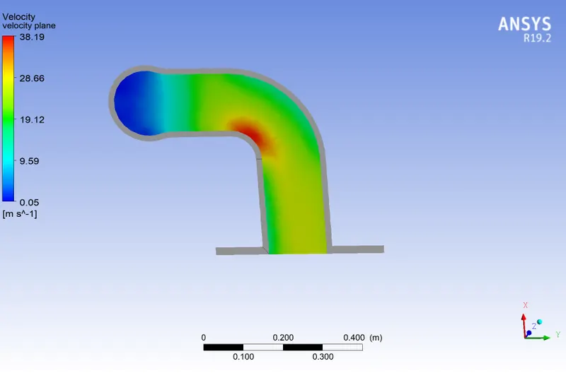
Velocity plot for base mesh,
Dtream line plot for base mesh,
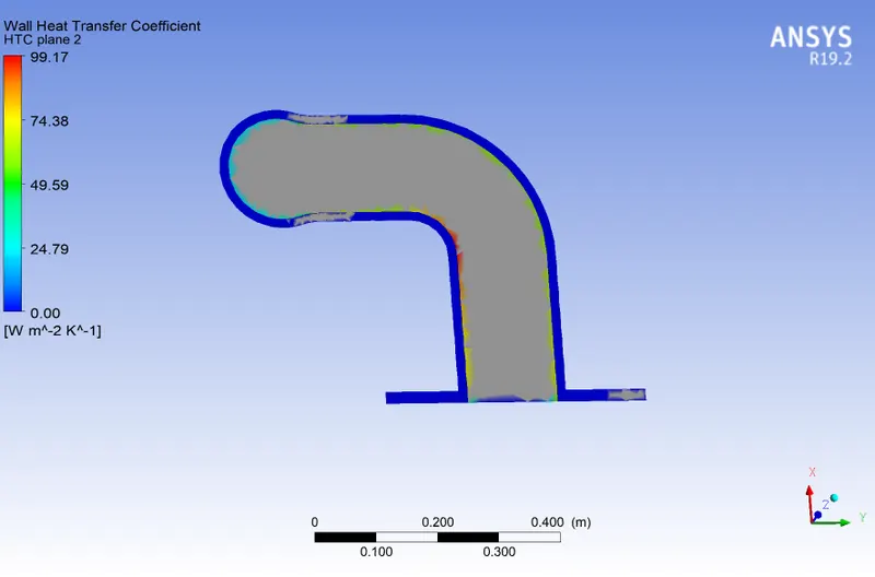
Heat Transfer Coefficient for Base mesh,
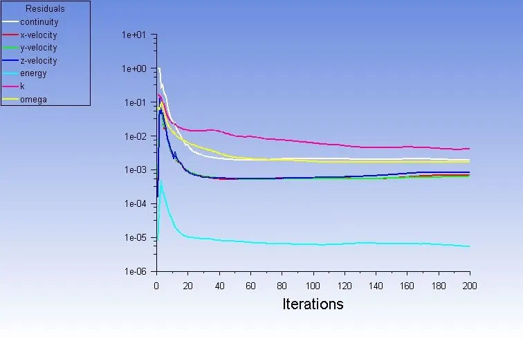
Residual plot for Refined mesh,
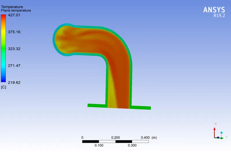
Temperature distribution plot for refined Mesh,
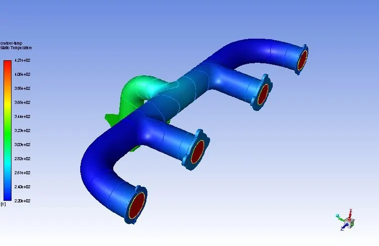
Temperature plot for Refined mesh,
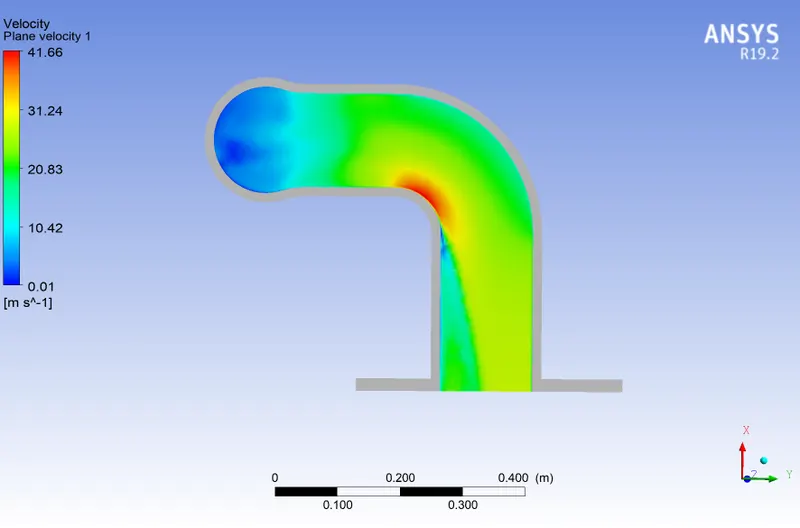
Velocity plot for Refined Mesh,
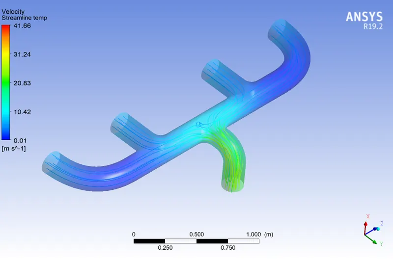
Streamline plot for Refined mesh,
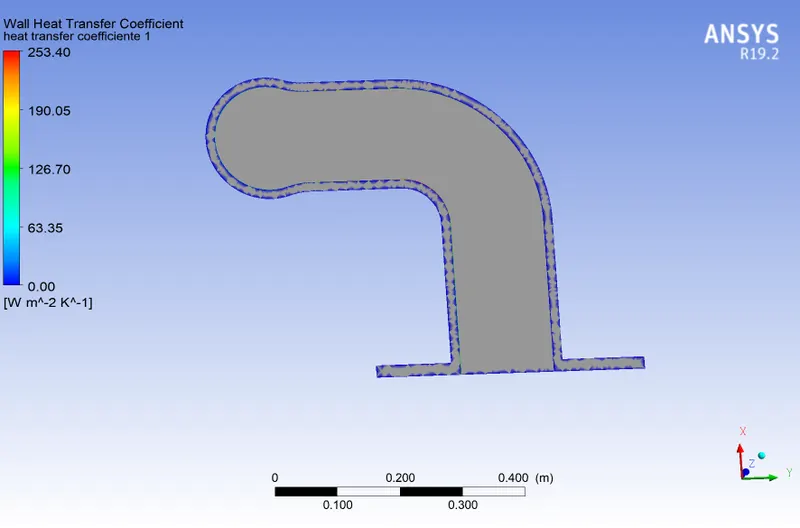
Heat transfer Coefficient plot for Refined Mesh,
To verify the HTC predictions from the simulations,
To verify the heat transfer Coefficient from the simulation it is necessary to perform the analytical calculation. This can be done by using the formula of nusselt number Nu=hl/k where h is heat transfer coefficient, l be the length and K the thermal conductivity of the material. So inorder to find h i.e heat transfer coefficient we need to find nusselt number.This can be done Using Dittus-Boelter Equation.
The equation is as follows:
Nu=0.023*(Reynolds number^(4/5))*(pr^n)
Where Nu is the nusselt number, pr is the prandtl number and n is 0.4 for the hot fluid or 0.3 for the cold fluid, From these two equations we can find the heat transfer coefficient and validate with the simulation result.
Factors depending the accuracy of the prediction are,
Clean geometry - Geometry with no errors and open surfaces
Mesh Refinement: The finer mesh simulation will have the approximate value closer to the experimental value.
Solver selection:Selecting the models wisely which is suitable for the application will get good result and less computational time. (In this case K-Omega SST is chosen over K-Epsilon where flow around the walls needs to captured).
Inflaation Layers - The first layer thickness around the walls should be provided for better accuracy.
Number of Iteration - The more complex the model is the time taken to converge the solution.
Conclusion
In conclusion , the solution obtained from the base mesh with no inflation layers shows inaccurate results since the mesh is not refined around the walls,whereas the solution and temperature plots and heat transfer coeffficient plot shows the good approximate results around the walls.Hence, conjugate heat transfer simulation for exhaust port is done and the solution for differeent cases is compared.